2 Data visualization

Prerequisites

library(tidyverse)
#> ── Attaching core tidyverse packages ───────────────────── tidyverse 2.0.0 ──
#> ✔ dplyr     1.1.2     ✔ readr     2.1.4
#> ✔ forcats   1.0.0     ✔ stringr   1.5.0
#> ✔ ggplot2   3.4.2     ✔ tibble    3.2.1
#> ✔ lubridate 1.9.2     ✔ tidyr     1.3.0
#> ✔ purrr     1.0.1     
#> ── Conflicts ─────────────────────────────────────── tidyverse_conflicts() ──
#> ✖ dplyr::filter() masks stats::filter()
#> ✖ dplyr::lag()    masks stats::lag()
#> ℹ Use the conflicted package (<http://conflicted.r-lib.org/>) to force all conflicts to become errors
library(palmerpenguins)

2.2.5 Exercises

There are 344 rows and 8 columns in the penguins data frame.
The bill_depth_mm denotes the bill depth in millimeters.

There is a positive, linear, and somewhat strong association between bill depth and bill length of penguins.

ggplot(
  data = penguins, 
  aes(x = bill_depth_mm, y = bill_length_mm)
) + 
  geom_point()
#> Warning: Removed 2 rows containing missing values (`geom_point()`).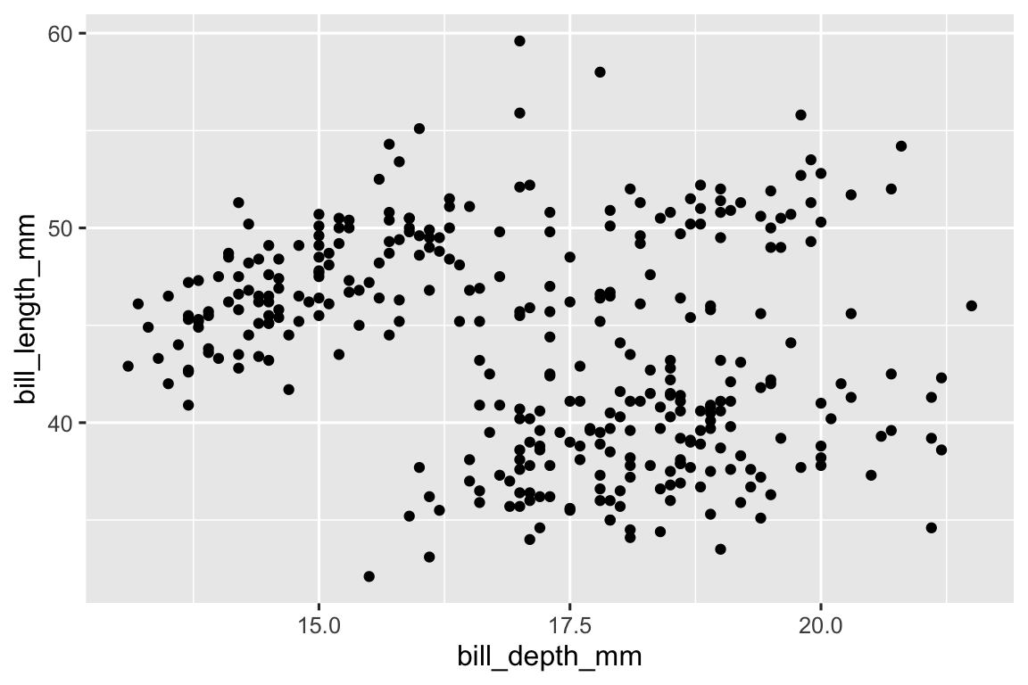

Species is a categorical variable and a scatterplot of a categorical variable is not that useful as it’s difficult to use it to describe the distribution of bill depth across species.
```
ggplot(
  data = penguins, 
  aes(x = bill_depth_mm, y = species)
) + 
  geom_point()
#> Warning: Removed 2 rows containing missing values (`geom_point()`).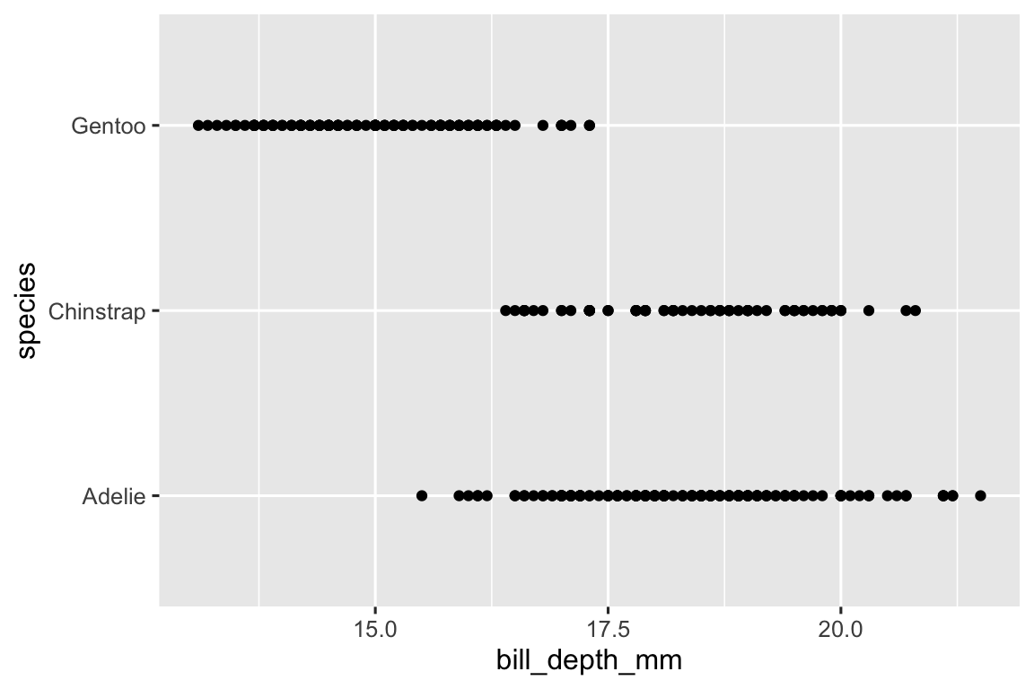
```

No aesthetic mappings for x and y are provided and these are required aesthetics for the point geom.

ggplot(data = penguins) + 
  geom_point()
#> Error in `geom_point()`:
#> ! Problem while setting up geom.
#> ℹ Error occurred in the 1st layer.
#> Caused by error in `compute_geom_1()`:
#> ! `geom_point()` requires the following missing aesthetics: x and y

Setting the na.rm argument to TRUE removes the missing values without a warning. The value for this argument is FALSE by default.

ggplot(
  data = penguins, 
  aes(x = bill_depth_mm, y = bill_length_mm)
) + 
  geom_point(na.rm = TRUE)

The plot from the previous exercise with caption added is provided below.

ggplot(
  data = penguins,
  aes(x = bill_depth_mm, y = bill_length_mm)
) +
  geom_point(na.rm = TRUE) +
  labs(caption = "Data come from the palmerpenguins package.")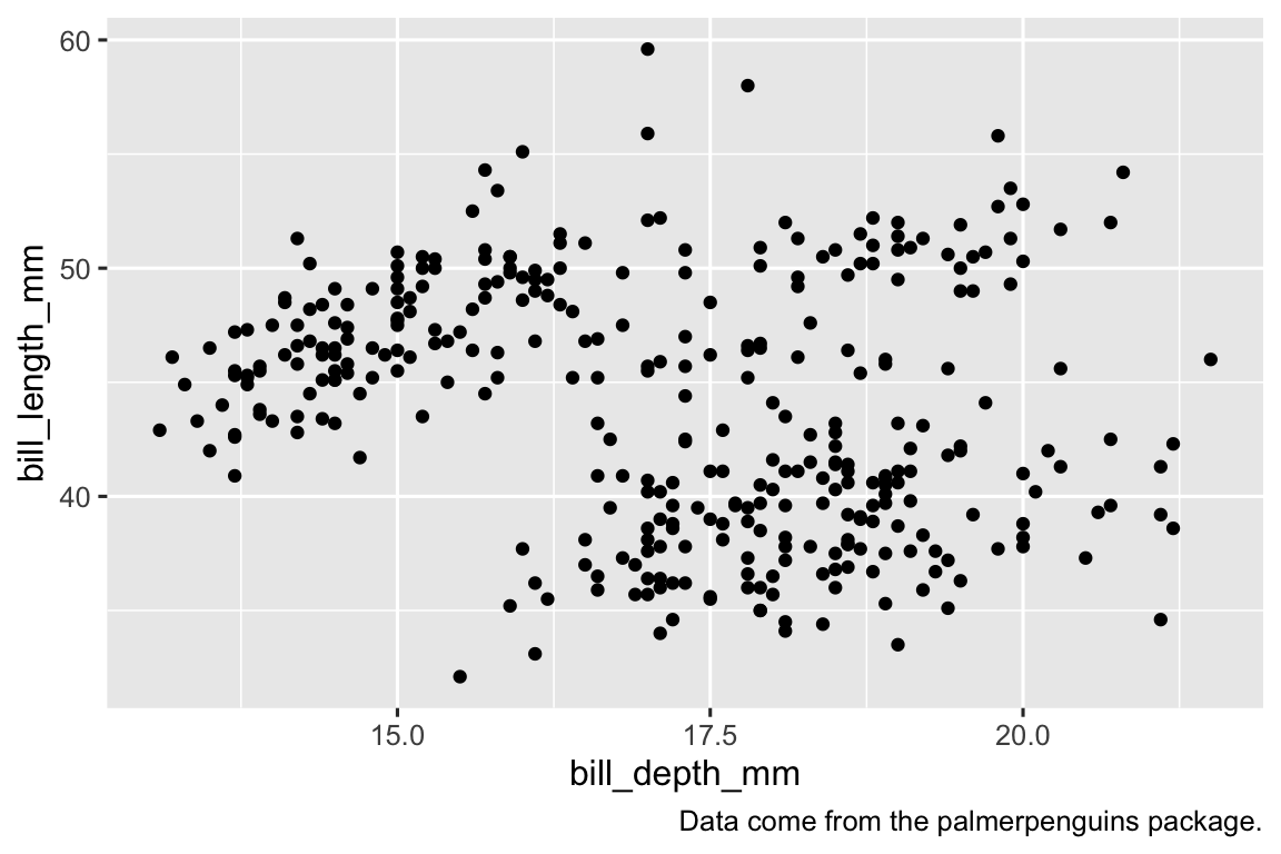

The code for recreating the visualization is provided below. The bill_depth_mm variable should be mapped at the local level, only for the point geom, as it is not used for the smooth geom – the points are colored for bill depth but the smooth line is a single color.

ggplot(
  data = penguins,
  aes(x = flipper_length_mm, y = body_mass_g)
) +
  geom_point(aes(color = bill_depth_mm)) + 
  geom_smooth()
#> `geom_smooth()` using method = 'loess' and formula = 'y ~ x'
#> Warning: Removed 2 rows containing non-finite values (`stat_smooth()`).
#> Warning: Removed 2 rows containing missing values (`geom_point()`).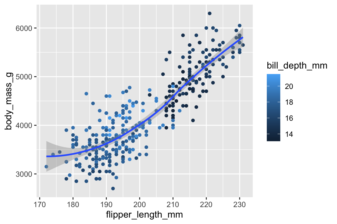

I would expect the a scatterplot of body mass vs. flipper length with points and smooth lines for each species in a different color. The plot below indeed shows this.

ggplot(
  data = penguins,
  mapping = aes(x = flipper_length_mm, y = body_mass_g, color = island)
) +
  geom_point() +
  geom_smooth(se = FALSE)
#> `geom_smooth()` using method = 'loess' and formula = 'y ~ x'
#> Warning: Removed 2 rows containing non-finite values (`stat_smooth()`).
#> Warning: Removed 2 rows containing missing values (`geom_point()`).

The two plots will look the same as in the first plot the aesthetic mappings are at the global level and passed down to both geoms, and in the second plot both geoms have the same aesthetic mappings, each defined at the local level.

ggplot(
  data = penguins,
  mapping = aes(x = flipper_length_mm, y = body_mass_g)
) +
  geom_point() +
  geom_smooth()
#> `geom_smooth()` using method = 'loess' and formula = 'y ~ x'
#> Warning: Removed 2 rows containing non-finite values (`stat_smooth()`).
#> Warning: Removed 2 rows containing missing values (`geom_point()`).

ggplot() +
  geom_point(
    data = penguins,
    mapping = aes(x = flipper_length_mm, y = body_mass_g)
  ) +
  geom_smooth(
    data = penguins,
    mapping = aes(x = flipper_length_mm, y = body_mass_g)
  )
#> `geom_smooth()` using method = 'loess' and formula = 'y ~ x'
#> Warning: Removed 2 rows containing non-finite values (`stat_smooth()`).
#> Removed 2 rows containing missing values (`geom_point()`).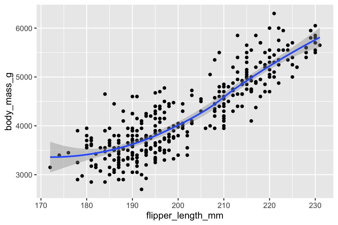

2.4.3 Exercises

This code makes the bars horizontal instead of vertical.

ggplot(penguins, aes(y = species)) + 
  geom_bar()

In the first plot, the borders of the bars are colored. In the second plot, the bars are filled in with colors. The fill aesthetic is more useful for changing the color of the bars.
```
ggplot(penguins, aes(x = species)) +
  geom_bar(color = "red")

ggplot(penguins, aes(x = species)) +
  geom_bar(fill = "red")
```
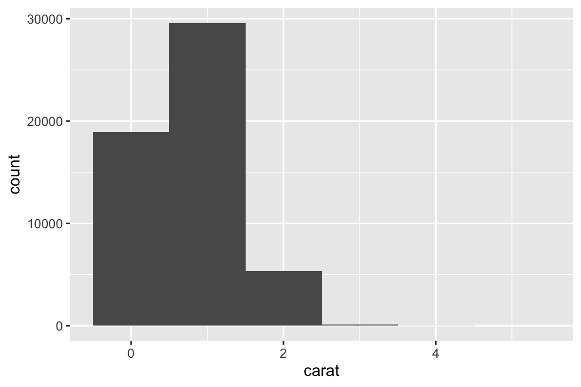
It determines the number of bins (bars) in a histogram.

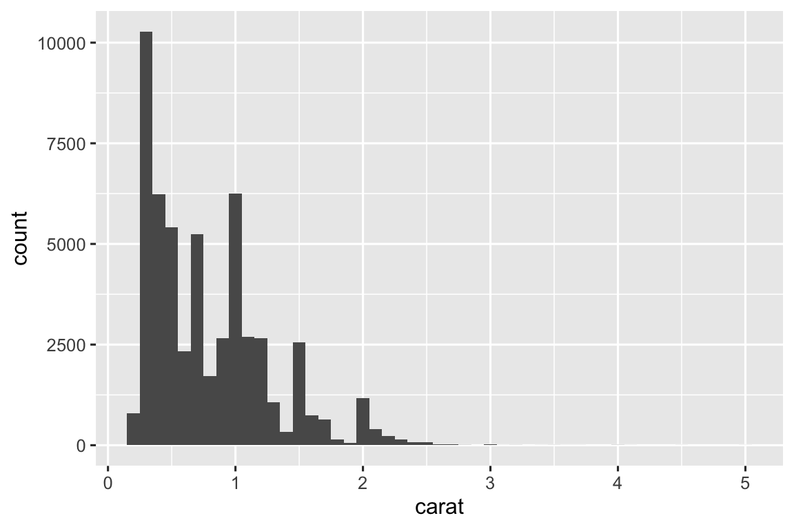
Below are histograms with three different binwidths. I think a binwidth of 0.10 shows reveals the most interesting patterns.

ggplot(diamonds, aes(x = carat)) +
  geom_histogram(binwidth = 0.01)

ggplot(diamonds, aes(x = carat)) +
  geom_histogram(binwidth = 0.10)

ggplot(diamonds, aes(x = carat)) +
  geom_histogram(binwidth = 1)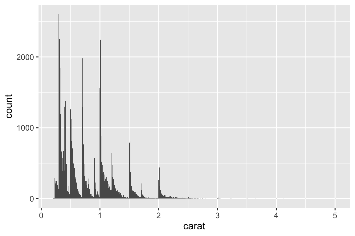

2.5.5 Exercises

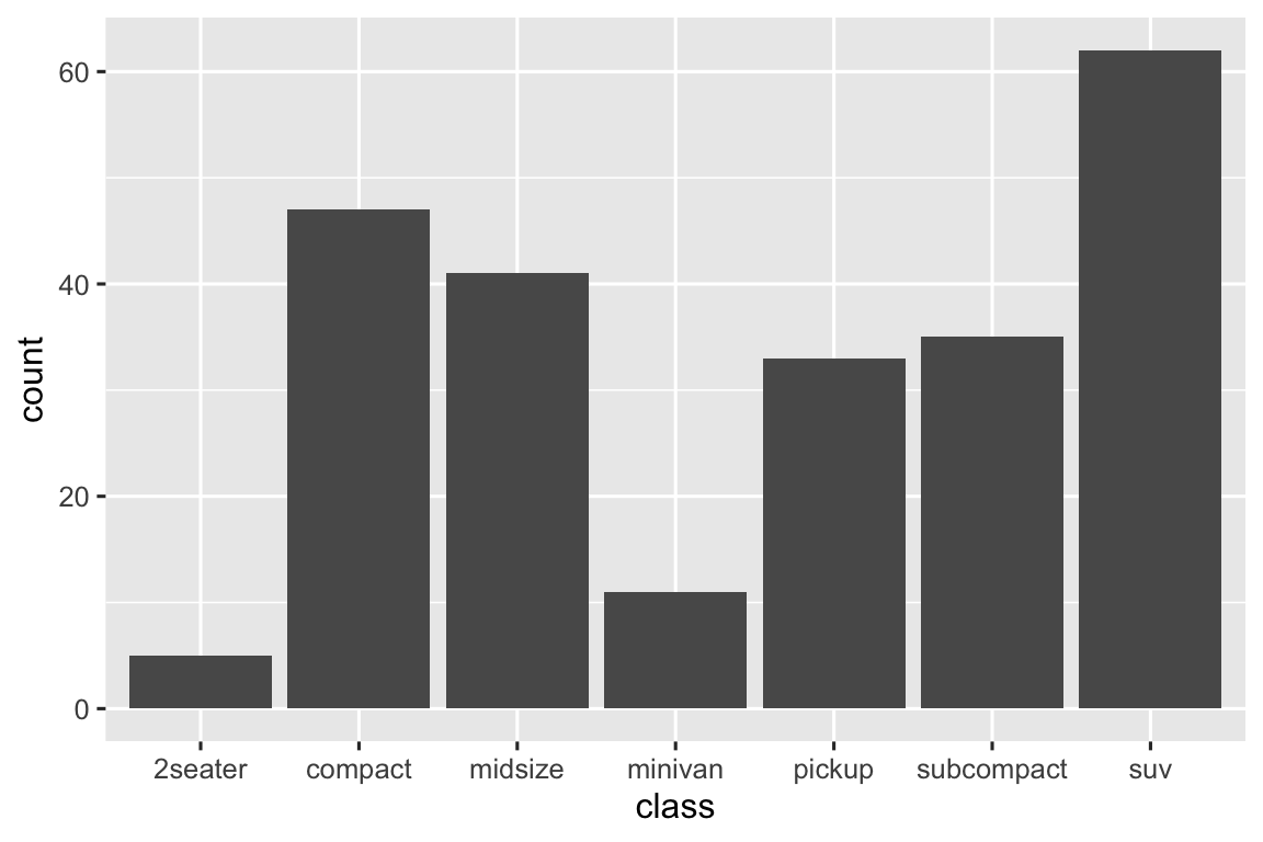
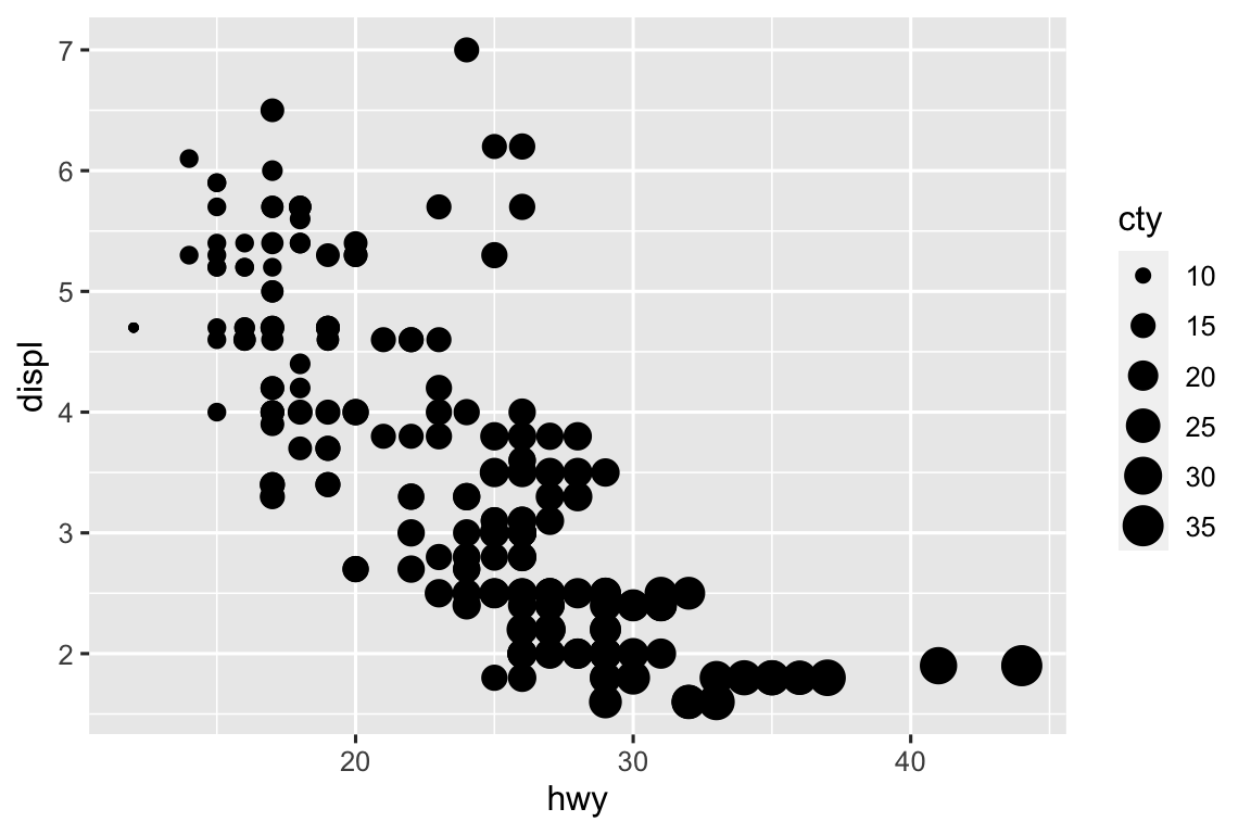
manufacturer, class, fl, drv, model, and trans are all categorical variables. displ, year, cyl, cty, and hwy are all numerical variables. You can run glimpse(mpg) or ?mpg to see a list of the variables.

The difference is a numerical variable doesn’t work with shape aesthetic but a categorical variable does. Also, the color scale is different for numerical and categorical variables.

ggplot(
  mpg, 
  aes(x = hwy, y = displ, color = cty)
) + 
  geom_point()

ggplot(
  mpg, 
  aes(x = hwy, y = displ, size = cty)
) + 
  geom_point()

ggplot(
  mpg, 
  aes(x = hwy, y = displ, size = cty, color = cty)
) + 
  geom_point()

ggplot(
  mpg, 
  aes(x = hwy, y = displ, size = cty, color = cty, shape = drv)
) + 
  geom_point()

Since there is no line to alter the width of, nothing happens. The code runs as though that aesthetic was not specified.
```
ggplot(mpg, aes(x = hwy, y = displ, linewidth = cty)) + 
  geom_point()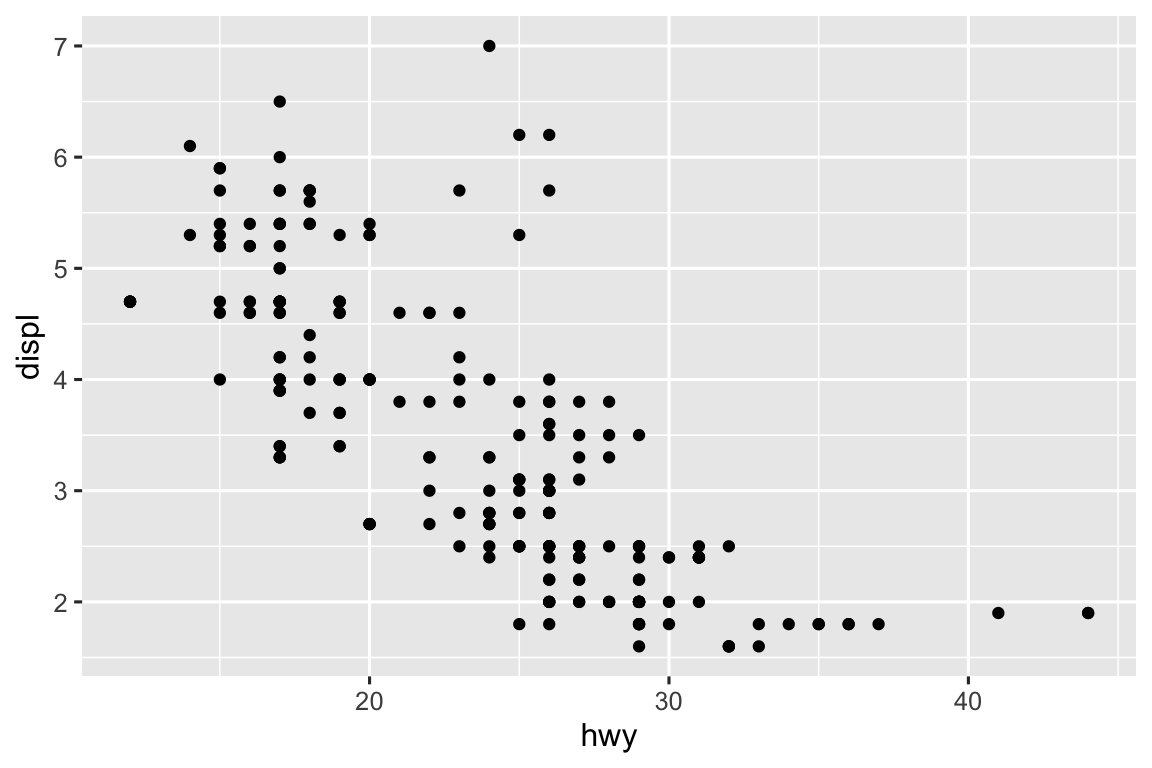
```
See below for a sample plot that maps hwy to x, yy, and color aesthetics. ggplot2 will allow you to map the same variable to multiple aesthetics, but the resulting plot is not useful.
```
ggplot(mpg, aes(x = hwy, y = hwy, color = hwy)) + 
  geom_point()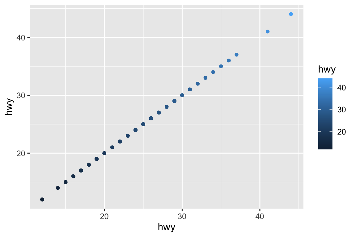
```

Adelies tend to have higher bill depth while Gentoo have longer bills and Chinstrap have deeper and longer bills.

ggplot(
  penguins,
  aes(x = bill_depth_mm, y = bill_length_mm, color = species)
) + 
  geom_point()
#> Warning: Removed 2 rows containing missing values (`geom_point()`).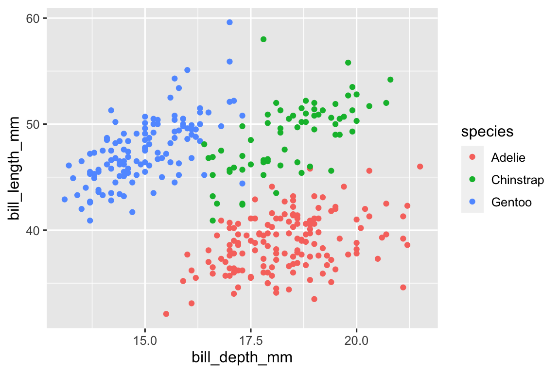

The code provided in the exercise yields two separate legends because the legend for color is renamed to "Species" but the legend for shape is not, and is named "species" by default instead. To fix it, we would need to explicitly rename the shape legend as well.

ggplot(
  data = penguins,
  mapping = aes(
    x = bill_length_mm, y = bill_depth_mm, 
    color = species, shape = species
  )
) +
  geom_point() +
labs(
  color = "Species",
  shape = "Species"
)
#> Warning: Removed 2 rows containing missing values (`geom_point()`).

2.6.1 Exercises

The second plot is saved, because ggsave() saves the last plot you made.

ggplot(mpg, aes(x = class)) +
  geom_bar()

ggplot(mpg, aes(x = cty, y = hwy)) +
  geom_point()

ggsave("mpg-plot.png")
#> Saving 6 x 4 in image

You need to change the suffix of the file from png to pdf in the ggsave() call.