class: center, middle, inverse, title-slide # Data Visualization in R with ggplot2 ## University of Cincinnati ### Mine Çetinkaya-Rundel ### 16 April 2019 <br><br> rstd.io/uoc-ggplot2-slides --- class: center, middle # Data visualization --- ## Data visualization > *"The simple graph has brought more information to the data analyst’s mind than any other device." > — John Tukey* - Data visualization is the creation and study of the visual representation of data. - Many tools for visualizing data (R is one of them) - Many approaches/systems within R for making data visualizations, **ggplot2** is one of them --- ## ggplot2 `\(\in\)` tidyverse .pull-left[ <img src="../img/ggplot2-part-of-tidyverse.png" width="80%" /> ] .pull-right[ - **ggplot2**: tidyverse's data visualization package - `gg` in "ggplot2" stands for Grammar of Graphics - Inspired by the book **Grammar of Graphics** by Leland Wilkinson - A grammar of graphics is a tool that enables concise description of components of a graphic <img src="../img/grammar-of-graphics.png" width="80%" /> ] --- ## Following along... .pull-left[ ### Option 1: RStudio local - Download the materials at https://rstd.io/uoc-ggplot2-repo and launch `uoc-ggplot2.Rproj` - Install `tidyverse` if you haven't done so before, or if you haven't updated it recently ```r install.packages("tidyverse") install.packages("ggrepel") ``` - Load the tidyverse ```r library(tidyverse) library(ggrepel) ``` - Open `ggplot2.Rmd` ] .pull-right[ ### Option 2: RStudio Cloud - Go to RStudio Cloud at https://rstd.io/uoc-ggplot2-cloud - Start the assignment called ggplot2 Workshop - Open the R Markdown file in the project called ggplot ] --- ## Datasets * Transit ride data + `daily`: daily summary of rides * Durham registered voter data + `durham_voters`: one row per voter ```r daily <- read_csv("../data/daily.csv") durham_voters <- read_csv("../data/durham_voters.csv") ``` --- class: center, middle # Layer up! --- <!-- --> --- **Exercise:** Which of the four datasets does this visualization use? Determine which variable is mapped to which aesthetic (x-axis, y-axis, etc.) element of the dataset. <!-- --> --- ## Basic ggplot2 syntax * DATA * MAPPING * GEOM --- ```r ggplot(data = daily) ``` <!-- --> --- ```r ggplot(data = daily, mapping = aes(x = ride_date, y = n_rides)) ``` <!-- --> --- ```r ggplot(data = daily, mapping = aes(x = ride_date, y = n_rides)) + geom_point() ``` <!-- --> --- ```r ggplot(data = daily, aes(x = ride_date, y = n_rides, color = day_of_week)) + geom_point() ``` <!-- --> --- ```r ggplot(data = daily, aes(x = ride_date, y = n_rides, color = day_of_week)) + geom_smooth() ``` ``` ## `geom_smooth()` using method = 'loess' and formula 'y ~ x' ``` <!-- --> --- ```r ggplot(data = daily, aes(x = ride_date, y = n_rides, color = day_of_week)) + geom_smooth(method = "loess") ``` <!-- --> --- ```r ggplot(data = daily, aes(x = ride_date, y = n_rides, color = day_of_week)) + geom_smooth(method = "loess", se = FALSE) ``` <!-- --> --- ```r ggplot(data = daily, aes(x = ride_date, y = n_rides, color = day_of_week)) + geom_smooth(method = "loess", se = FALSE) + scale_color_viridis_d() ``` <!-- --> --- ```r ggplot(data = daily, aes(x = ride_date, y = n_rides, color = day_of_week)) + geom_smooth(method = "loess", se = FALSE) + scale_color_viridis_d() + theme_minimal() ``` <!-- --> --- ```r ggplot(data = daily, aes(x = ride_date, y = n_rides, color = day_of_week)) + geom_smooth(se = FALSE, method = "loess") + scale_color_viridis_d() + theme_minimal() + labs(x = "Ride date", y = "Number of rides", color = "Day of week", title = "Daily rides", subtitle = "Durham, NC") ``` <!-- --> --- ## ggplot, the making of 1. "Initialize" a plot with ggplot() 2. Add layers with geom_ functions ``` ggplot(data = <DATA>) + <GEOM_FUNCTION>(mapping = aes(<MAPPINGS>))+ geom_point(mapping = aes(x = displ, y = hwy)) ``` --- class: center, middle # Mapping --- ## Size by number of riders ```r ggplot(data = daily, aes(x = ride_date, y = n_rides, size = n_riders)) + geom_point() ``` <!-- --> --- ## Set alpha value ```r ggplot(data = daily, aes(x = ride_date, y = n_rides, size = n_riders)) + geom_point(alpha = 0.5) ``` <!-- --> --- **Exercise:** Using information from https://ggplot2.tidyverse.org/articles/ggplot2-specs.html add color, size, alpha, and shape aesthetics to your graph. Experiment. Do different things happen when you map aesthetics to discrete and continuous variables? What happens when you use more than one aesthetic? ```r ggplot(data = daily, aes(x = ride_date, y = n_rides, color = day_of_week)) + geom_smooth(se = FALSE, method = "loess") + scale_color_viridis_d() + theme_minimal() + labs(x = "Ride date", y = "Number of rides", color = "Day of week", title = "Daily rides", subtitle = "Durham, NC") ``` --- <img src="../img/aesthetic-mappings.png" width="80%" /> --- ## Mappings can be at the `geom` level ```r ggplot(data = daily) + geom_point(mapping = aes(x = ride_date, y = n_rides)) ``` <!-- --> --- ## Different mappings for different `geom`s ```r ggplot(data = daily, mapping = aes(x = ride_date, y = n_rides)) + geom_point() + geom_smooth(aes(color = day_of_week), method = "loess", se = FALSE) ``` <!-- --> --- ## Set vs. map .pull-left[ To **map** an aesthetic to a variable, place it inside `aes()` ```r ggplot(data = daily, mapping = aes(x = ride_date, y = n_rides, color = day_of_week)) + geom_point() ``` <!-- --> ] .pull-right[ To **set** an aesthetic to a value, place it outside `aes()` ```r ggplot(data = daily, mapping = aes(x = ride_date, y = n_rides)) + geom_point(color = "red") ``` <!-- --> ] --- class: center, middle # Syntax --- ## Data can be passed in ```r daily %>% ggplot(aes(x = ride_date, y = n_rides)) + geom_point() ``` <!-- --> --- ## Parameters can be unnamed ```r ggplot(daily, aes(x = ride_date, y = n_rides)) + geom_point() ``` <!-- --> --- ## Variable creation on the fly... Color by weekday / weekend ```r ggplot(data = daily, aes(x = ride_date, y = n_rides, color = day_of_week %in% c("Sat", "Sun"))) + geom_point() ``` <!-- --> --- ## Variable creation on the fly... ```r ggplot(data = daily, aes(x = ride_date, y = n_rides, color = day_of_week %in% c("Sat", "Sun"))) + geom_point() + labs(color = "Weekend") ``` <!-- --> --- ## ... or passed in ```r daily %>% mutate(day_type = if_else(day_of_week %in% c("Sat", "Sun"), "Weekend", "Weekday")) %>% ggplot(aes(x = ride_date, y = n_rides, color = day_type)) + geom_point() ``` <!-- --> --- class: center, middle # Common early pitfalls --- ## Mappings that aren't ```r ggplot(data = daily) + geom_point(aes(x = ride_date, y = n_rides, color = "blue")) ``` <!-- --> --- ## Mappings that aren't ```r ggplot(data = daily) + geom_point(aes(x = ride_date, y = n_rides), color = "blue") ``` <!-- --> --- ## + and %>% **Exercise:** What is wrong with the following? ```r daily %>% mutate(day_type = if_else(day_of_week %in% c("Sat", "Sun"), "Weekend", "Weekday")) %>% ggplot(aes(x = ride_date, y = n_rides, color = day_type)) %>% geom_point() ``` --- ## + and %>% What is wrong with the following? ```r daily %>% mutate(day_type = if_else(day_of_week %in% c("Sat", "Sun"), "Weekend", "Weekday")) %>% ggplot(aes(x = ride_date, y = n_rides, color = day_type)) %>% geom_point() ``` ``` ## Error: `mapping` must be created by `aes()` ## Did you use %>% instead of +? ``` --- class: center, middle # Building up layer by layer --- ## Basic plot ```r ggplot(data = daily, aes(x = ride_date, y = n_rides)) + geom_point() ``` <!-- --> --- ## Two layers! ```r ggplot(data = daily, aes(x = ride_date, y = n_rides)) + geom_point() + geom_line() ``` <!-- --> --- ## Iterate on layers ```r ggplot(data = daily, aes(x = ride_date, y = n_rides)) + geom_point() + geom_smooth(span = 0.1) # try changing span ``` ``` ## `geom_smooth()` using method = 'loess' and formula 'y ~ x' ``` <!-- --> --- ## The power of groups ```r ggplot(data = daily, aes(x = ride_date, y = n_rides, color = day_of_week)) + geom_point() + geom_line() ``` <!-- --> --- ## Now we've got it ```r ggplot(data = daily, aes(x = ride_date, y = n_rides, color = day_of_week)) + geom_smooth(span = 0.2, se = FALSE) ``` ``` ## `geom_smooth()` using method = 'loess' and formula 'y ~ x' ``` <!-- --> --- ## Control data by layer ```r ggplot(data = daily, aes(x = ride_date, y = n_rides, color = day_of_week)) + geom_point(data = filter(daily, !(day_of_week %in% c("Sat", "Sun")) & n_rides < 200), size = 5, color = "gray") + geom_point() ``` <!-- --> --- **Exercise:** Work with your neighbor to sketch what the following plot will look like. No cheating! Do not run the code, just think through the code for the time being. ```r low_weekdays <- daily %>% filter(!(day_of_week %in% c("Sat", "Sun")) & n_rides < 100) ggplot(daily, aes(x = ride_date, y = n_rides, color = day_of_week)) + geom_point(data = low_weekdays, size = 5, color = "gray") + geom_point() + geom_text(data = low_weekdays, aes(y = n_rides + 15, label = ride_date), size = 2, color = "black") ``` --- ```r low_weekdays <- daily %>% filter(!(day_of_week %in% c("Sat", "Sun")) & n_rides < 100) low_weekdays ``` ``` ## # A tibble: 9 x 7 ## ride_date day_of_week month n_rides n_riders n_unique_stops ## <date> <chr> <chr> <dbl> <dbl> <dbl> ## 1 2015-01-01 Thurs Jan 58 37 44 ## 2 2015-01-26 Mon Jan 58 52 15 ## 3 2015-01-28 Wed Jan 79 65 11 ## 4 2015-01-30 Fri Jan 25 25 12 ## 5 2015-02-03 Tues Feb 2 2 2 ## 6 2015-02-17 Tues Feb 46 34 33 ## 7 2015-02-26 Thurs Feb 30 22 22 ## 8 2015-05-25 Mon May 99 55 66 ## 9 2015-12-25 Fri Dec 1 1 1 ## # … with 1 more variable: n_unique_routes <dbl> ``` --- ```r ggplot(daily, aes(x = ride_date, y = n_rides, color = day_of_week)) + geom_point() ``` <!-- --> --- ```r ggplot(daily, aes(x = ride_date, y = n_rides, color = day_of_week)) + geom_point() + geom_point(data = low_weekdays, size = 5, color = "gray") ``` <!-- --> --- ```r ggplot(daily, aes(x = ride_date, y = n_rides, color = day_of_week)) + geom_point(data = low_weekdays, size = 5, color = "gray") + geom_point() ``` <!-- --> --- ```r ggplot(daily, aes(x = ride_date, y = n_rides, color = day_of_week)) + geom_point(data = low_weekdays, size = 5, color = "gray") + geom_point() + geom_text(data = low_weekdays, aes(y = n_rides, label = ride_date), size = 2, color = "black") ``` <!-- --> --- ```r ggplot(daily, aes(x = ride_date, y = n_rides, color = day_of_week)) + geom_point(data = low_weekdays, size = 5, color = "gray") + geom_point() + geom_text(data = low_weekdays, aes(y = n_rides + 15, label = ride_date), size = 2, color = "black") ``` <!-- --> --- ```r library(ggrepel) ggplot(daily, aes(x = ride_date, y = n_rides, color = day_of_week)) + geom_point(data = low_weekdays, size = 5, color = "gray") + geom_point() + geom_text_repel(data = low_weekdays, aes(x = ride_date, y = n_rides, label = as.character(ride_date)), size = 3, color = "black") ``` <!-- --> --- ```r ggplot(daily, aes(x = ride_date, y = n_rides, color = day_of_week)) + geom_point(data = low_weekdays, size = 5, color = "gray") + geom_point() + geom_label_repel(data = low_weekdays, aes(x = ride_date, y = n_rides, label = as.character(ride_date)), size = 2, color = "black") ``` <!-- --> --- **Exercise:** How would you fix the following plot? ```r ggplot(daily, aes(x = ride_date, y = n_rides, color = day_of_week)) + geom_smooth(color = "blue") ``` ``` ## `geom_smooth()` using method = 'loess' and formula 'y ~ x' ``` <!-- --> --- ## Other geoms - There are a number of other geoms besides `geom_point()`, `geom_line()`, `geom_smooth()`, and `geom_text()`. - More info: [ggplot2.tidyverse.org/reference](https://ggplot2.tidyverse.org/reference/) --- class: center, middle # Splitting over facets --- ## Data prep ```r daily <- daily %>% mutate( day = if_else(day_of_week %in% c("Sat", "Sun"), "Weekend", "Weekday"), temp = if_else(month %in% c("Jan", "Feb", "Mar", "Apr", "May", "Jun"), "Cooler", "Warmer") ) %>% select(day, temp, everything()) daily ``` ``` ## # A tibble: 364 x 9 ## day temp ride_date day_of_week month n_rides n_riders n_unique_stops ## <chr> <chr> <date> <chr> <chr> <dbl> <dbl> <dbl> ## 1 Week… Cool… 2015-01-01 Thurs Jan 58 37 44 ## 2 Week… Cool… 2015-01-02 Fri Jan 134 83 93 ## 3 Week… Cool… 2015-01-03 Sat Jan 145 84 100 ## 4 Week… Cool… 2015-01-04 Sun Jan 101 57 63 ## 5 Week… Cool… 2015-01-05 Mon Jan 182 117 109 ## 6 Week… Cool… 2015-01-06 Tues Jan 267 138 146 ## 7 Week… Cool… 2015-01-07 Wed Jan 243 157 129 ## 8 Week… Cool… 2015-01-08 Thurs Jan 235 154 141 ## 9 Week… Cool… 2015-01-09 Fri Jan 268 173 147 ## 10 Week… Cool… 2015-01-10 Sat Jan 198 114 116 ## # … with 354 more rows, and 1 more variable: n_unique_routes <dbl> ``` --- ## facet_wrap ```r ggplot(data = daily, aes(x = ride_date, y = n_rides)) + geom_line() + facet_wrap( ~ day) ``` <!-- --> --- ## facet_grid ```r ggplot(data = daily, aes(x = ride_date, y = n_rides)) + geom_line() + facet_grid(temp ~ day) ``` <!-- --> --- ## facet_grid ```r ggplot(data = daily, aes(x = ride_date, y = n_rides)) + geom_line() + facet_grid(day ~ temp) ``` <!-- --> --- ## Durham voters ```r durham_voters %>% select(race_code, gender_code, age) ``` ``` ## # A tibble: 204,063 x 3 ## race_code gender_code age ## <chr> <chr> <chr> ## 1 I M Age Over 66 ## 2 U U Age 18 - 25 ## 3 O F Age 41 - 65 ## 4 W F Age 41 - 65 ## 5 W M Age 41 - 65 ## 6 B M Age 26 - 40 ## 7 W F Age 41 - 65 ## 8 W M Age 26 - 40 ## 9 B F Age 41 - 65 ## 10 B M Age 41 - 65 ## # … with 204,053 more rows ``` --- ## Data prep ```r durham_voters %>% group_by(race_code, gender_code, age) %>% summarize(n_voters = n(), n_rep = sum(party == "REP")) ``` ``` ## # A tibble: 92 x 5 ## # Groups: race_code, gender_code [21] ## race_code gender_code age n_voters n_rep ## <chr> <chr> <chr> <int> <int> ## 1 A F Age < 18 Or Invalid Birth Date 2 0 ## 2 A F Age 18 - 25 751 35 ## 3 A F Age 26 - 40 1086 64 ## 4 A F Age 41 - 65 727 75 ## 5 A F Age Over 66 170 36 ## 6 A M Age 18 - 25 635 42 ## 7 A M Age 26 - 40 919 64 ## 8 A M Age 41 - 65 572 61 ## 9 A M Age Over 66 175 33 ## 10 A U Age 18 - 25 8 1 ## # … with 82 more rows ``` --- ## Data prep ```r durham_voters_summary <- durham_voters %>% group_by(race_code, gender_code, age) %>% summarize(n_all_voters = n(), n_rep_voters = sum(party == "REP")) %>% filter(gender_code %in% c("F", "M") & race_code %in% c("W", "B", "A") & age != "Age < 18 Or Invalid Birth Date") ``` --- ## facet_grid ```r ggplot(durham_voters_summary, aes(x = age, y = n_all_voters)) + geom_bar(stat = "identity") + facet_grid(race_code ~ gender_code) ``` <!-- --> --- ## Free scales ```r ggplot(durham_voters_summary, aes(x = age, y = n_all_voters)) + geom_bar(stat = "identity") + facet_grid(race_code ~ gender_code, scales = "free_y") ``` <!-- --> --- ## Facets + layers 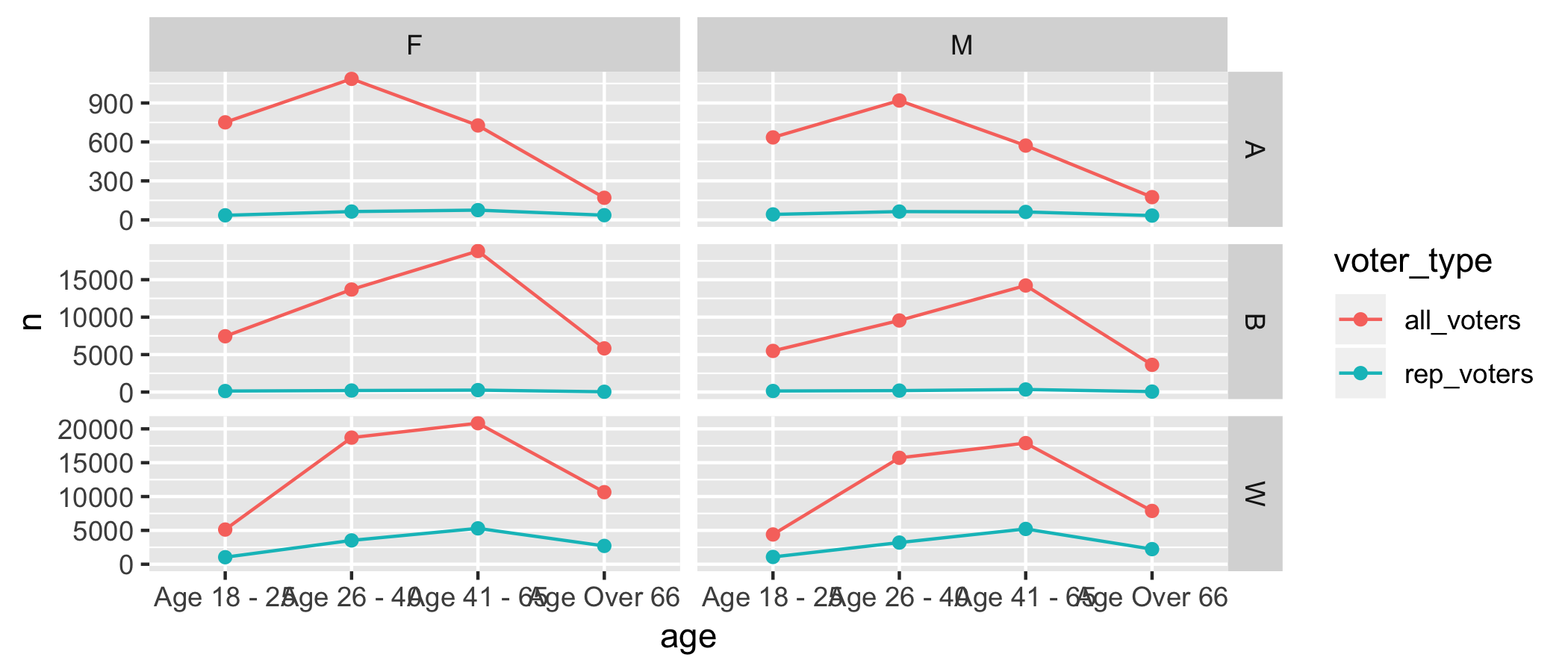<!-- --> --- ## Facets + layers Using new tidyr function: `pivot_longer()` ```r durham_voters_summary %>% tidyr::pivot_longer(cols = starts_with("n_"), names_to = "voter_type", values_to = "n", names_prefix = "n_") %>% mutate(age_cat = as.numeric(as.factor(age))) %>% ggplot(aes(x = age, y = n, color = voter_type)) + geom_point() + geom_line(aes(x = age_cat)) + facet_grid(race_code ~ gender_code, scales = "free_y") + expand_limits(y = 0) ``` --- class: center, middle # Scales and legends --- ## Scale transformation ```r ggplot(data = daily, aes(x = ride_date, y = n_rides, color = day_of_week)) + geom_point() + scale_y_reverse() ``` 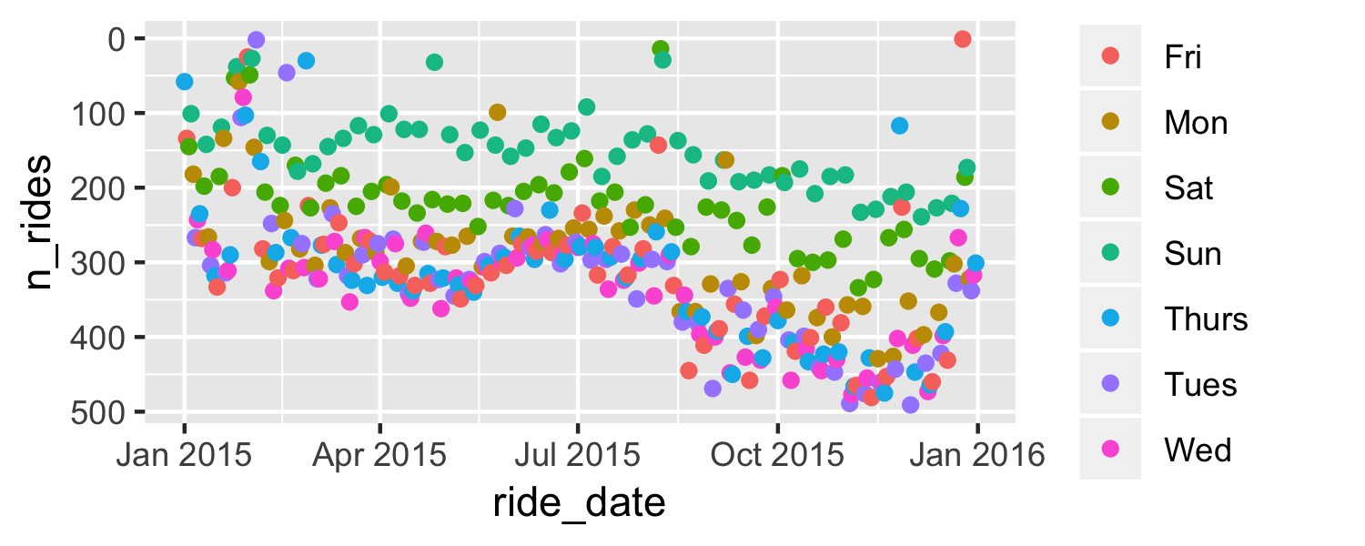<!-- --> --- ## Scale transformation ```r ggplot(data = daily, aes(x = ride_date, y = n_rides, color = day_of_week)) + geom_point() + scale_y_sqrt() ``` 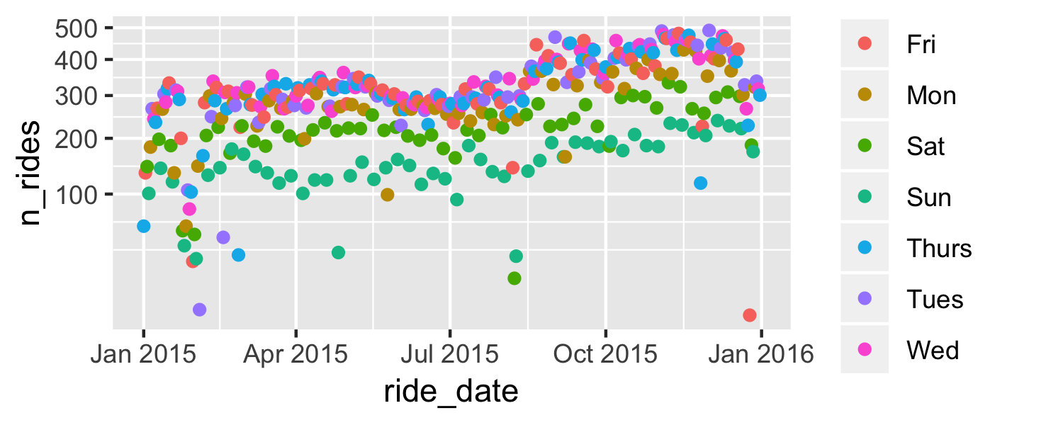<!-- --> --- ## Scale details ```r ggplot(data = daily, aes(x = ride_date, y = n_rides, color = day_of_week)) + geom_point() + scale_y_continuous(breaks = c(0, 200, 500)) ``` 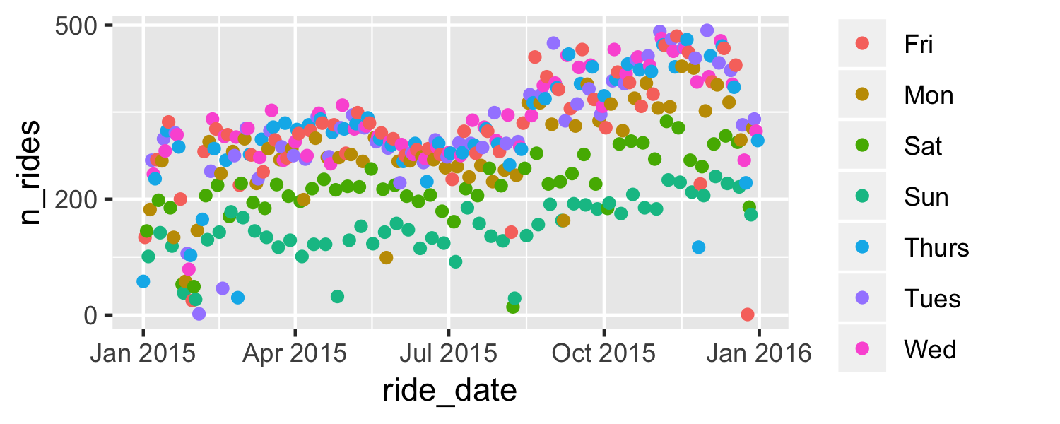<!-- --> --- class: center, middle # Themes and refinements --- ## Overall themes ```r ggplot(data = daily, aes(x = ride_date, y = n_rides, color = day_of_week)) + geom_point() + theme_bw() ``` <!-- --> --- ## Overall themes ```r ggplot(data = daily, aes(x = ride_date, y = n_rides, color = day_of_week)) + geom_point() + theme_dark() ``` <!-- --> --- ## Customizing theme elements ```r ggplot(data = daily, aes(x = ride_date, y = n_rides, color = day_of_week)) + geom_point() + theme(axis.text.x = element_text(angle = 90)) ``` <!-- --> --- **Exercise:** Fix the axis labels in the following plot so they don't overlap by playing around with their orientation. ```r ggplot(durham_voters_summary, aes(x = age, y = n_all_voters)) + geom_bar(stat = "identity") + facet_grid(race_code ~ gender_code, scales = "free_y") ``` <!-- --> --- ## Themes Vignette To really master themes: [ggplot2.tidyverse.org/articles/extending-ggplot2.html#creating-your-own-theme](https://ggplot2.tidyverse.org/articles/extending-ggplot2.html#creating-your-own-theme) --- class: center, middle # Recap --- ## The basics * map variables to aethestics * add "geoms" for visual representation layers * scales can be independently managed * legends are automatically created * statistics are sometimes calculated by geoms --- ## ggplot2 template Make any plot by filling in the parameters of this template ```r knitr::include_graphics("../img/ggplot2-template.png") ``` <img src="../img/ggplot2-template.png" width="100%" /> --- ## Learn more * Books: - [R for Data Science](https://r4ds.had.co.nz) by Grolemund and Wickham - [R Graphics Cookbook](http://www.cookbook-r.com/Graphs/) by Chang - [Data Visualization: A Practical Introduction](https://kieranhealy.org/publications/dataviz/) by Healy * [ggplot2.tidyverse.org](https://ggplot2.tidyverse.org/) * [ggplot2 Cheat sheet](https://github.com/rstudio/cheatsheets/blob/master/data-visualization-2.1.pdf) * Contributed extensions: [ggplot2-exts.org](http://www.ggplot2-exts.org/) --- ## Thanks Thanks to Elaine McVey and Sheila Saia for sharing their slides from previous R-Ladies RTP meetups!