setting the scene

Assumption 1:
Teach authentic tools

Assumption 2:
Teach R as the authentic tool
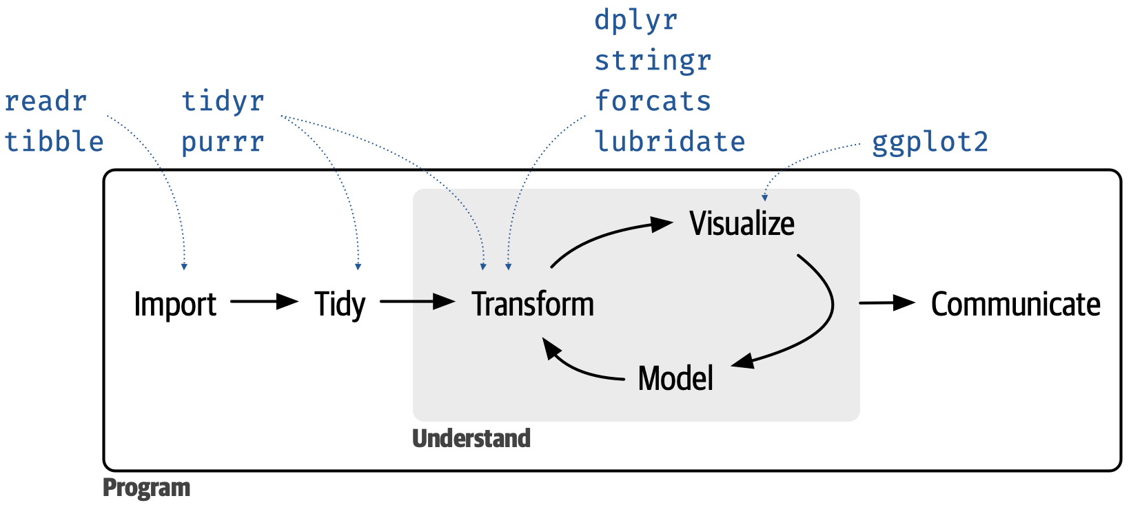
tidyverse
- meta R package that loads eight core packages when invoked and also bundles numerous other packages upon installation
- tidyverse packages share a design philosophy, common grammar, and data structures
task: data visualization
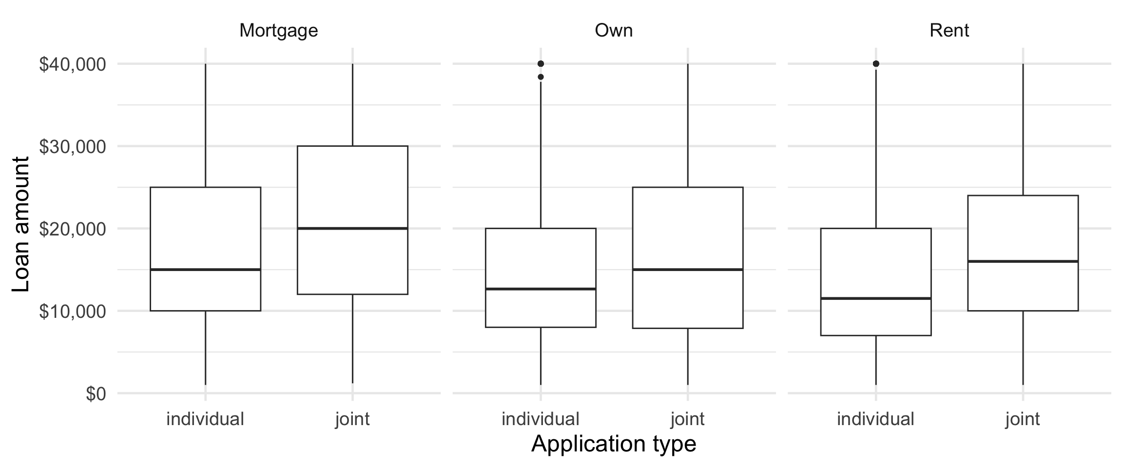
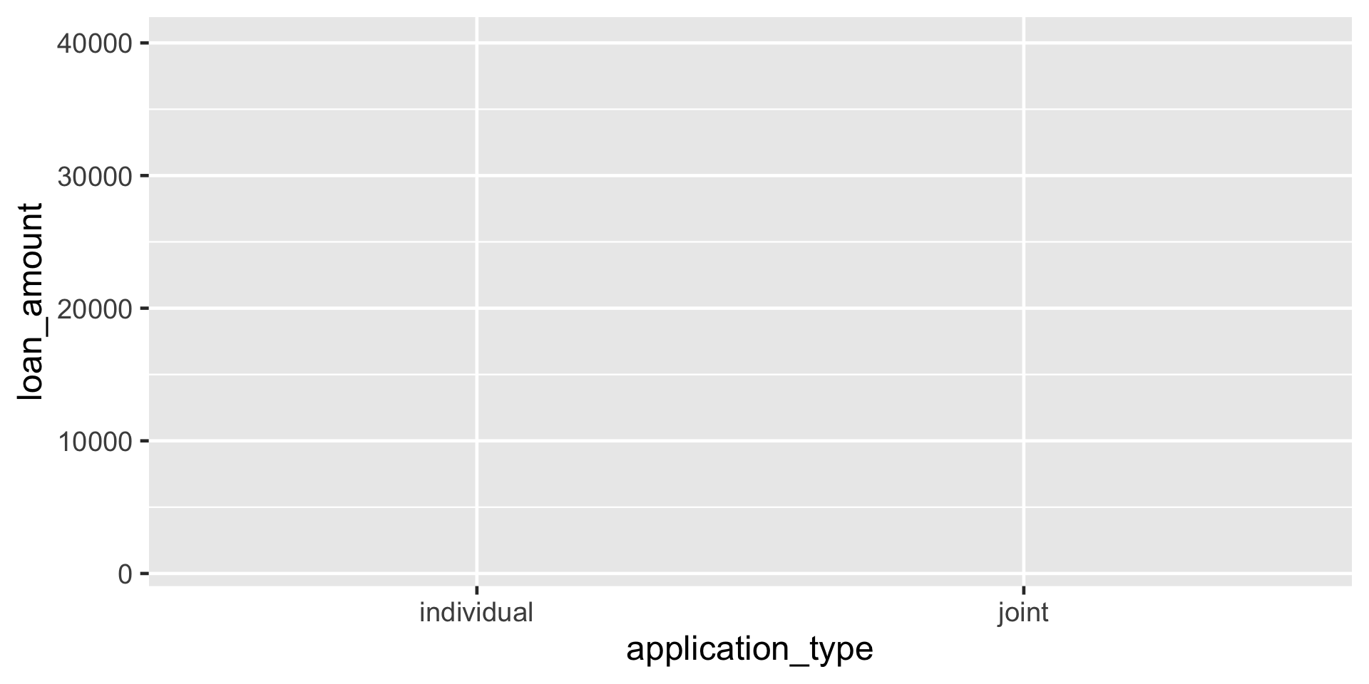
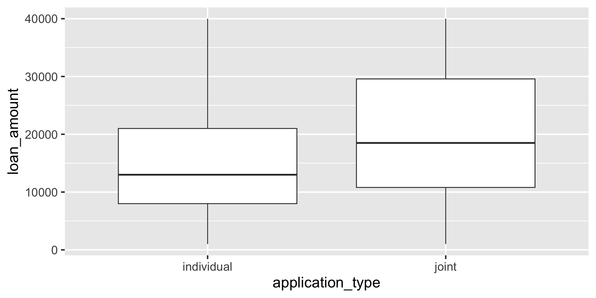
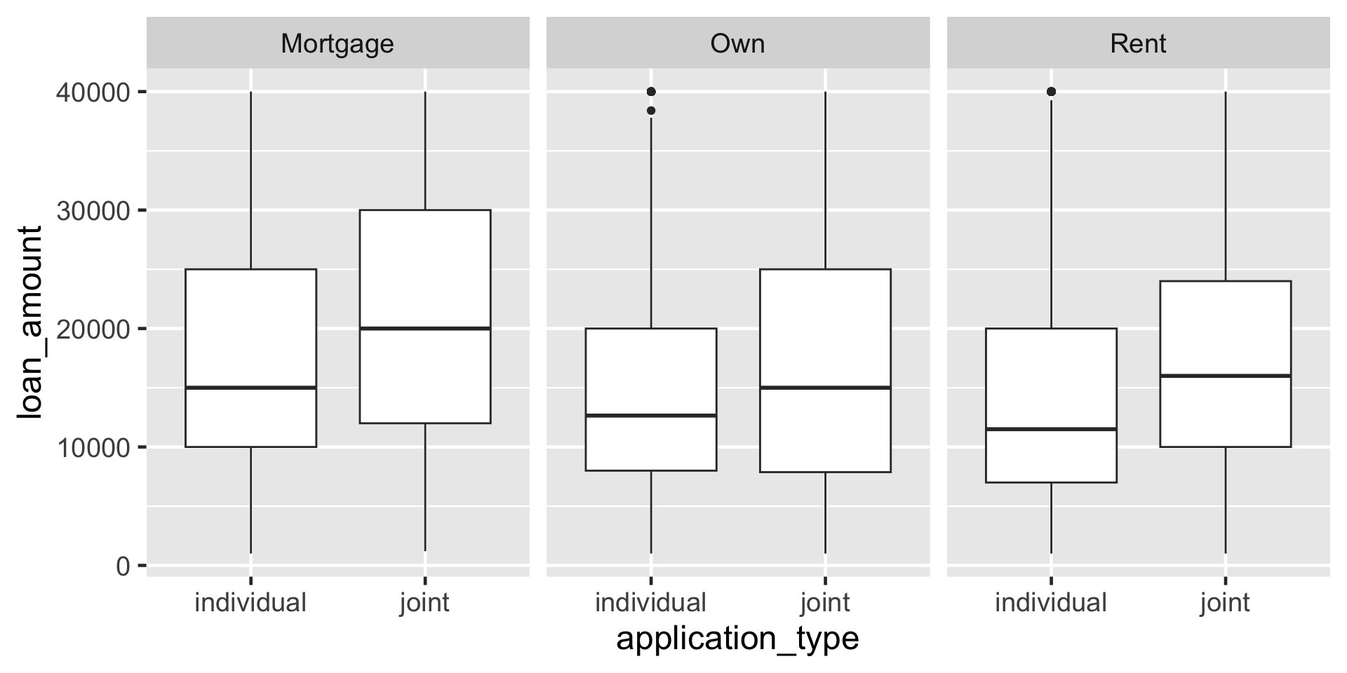
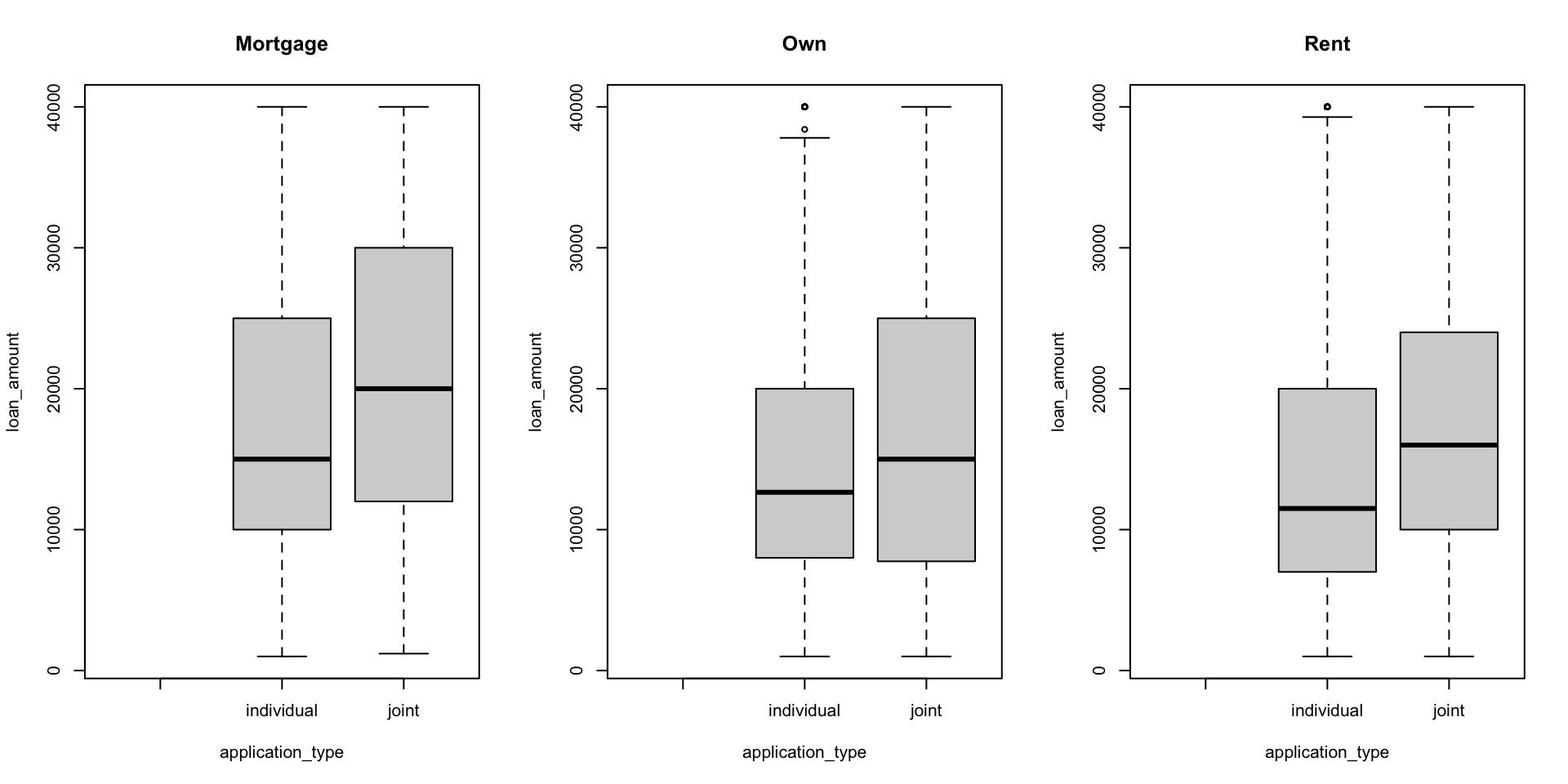
Create side-by-side box plots that shows the relationship between loan amount and application type, faceted by homeownership.
break it down I

break it down II
break it down III
break it down IV
break it down IV
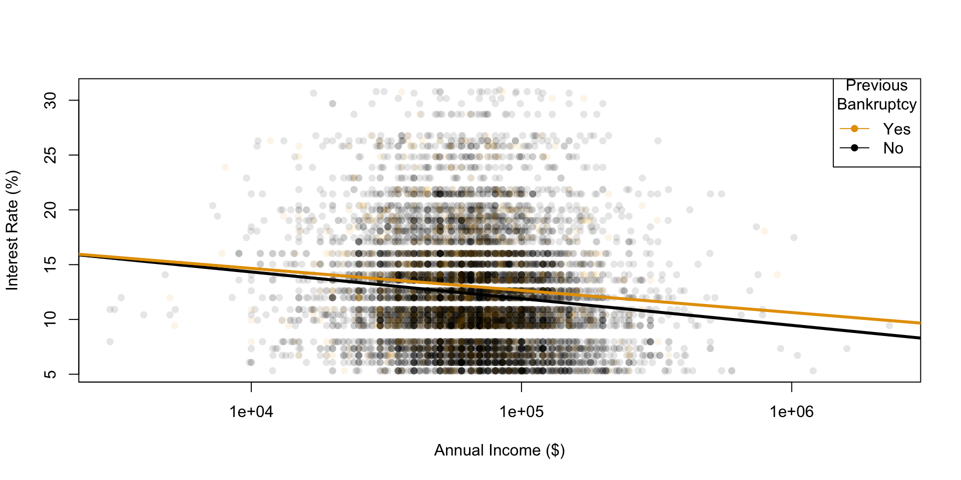
plotting with boxplot()
visualizing a different relationship
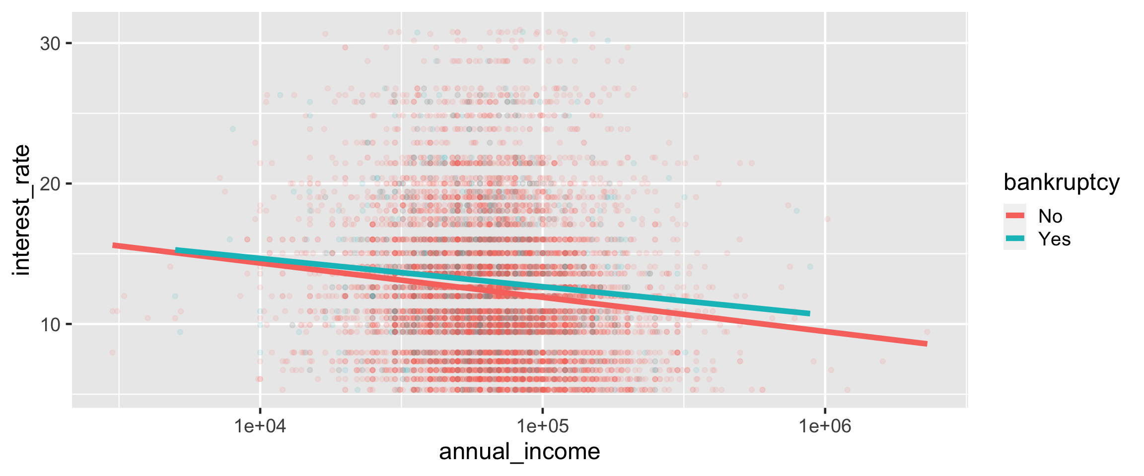
Visualize the relationship between interest rate and annual income, conditioned on whether the applicant had a bankruptcy.
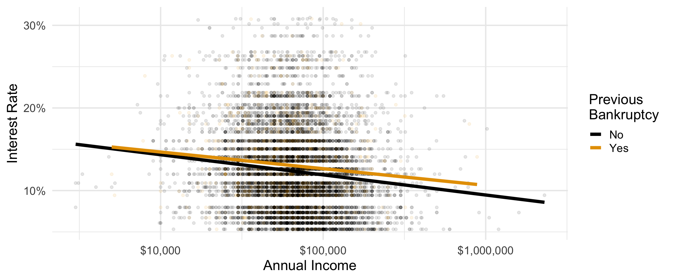
plotting with ggplot()
further customizing ggplot()
ggplot(loans,
       aes(y = interest_rate, x = annual_income,
           color = bankruptcy)) +
  geom_point(alpha = 0.1) +
  geom_smooth(method = "lm", size = 2, se = FALSE) +
  scale_x_log10(labels = scales::label_dollar()) +
  scale_y_continuous(labels = scales::label_percent(scale = 1)) +
  scale_color_colorblind() +
  labs(x = "Annual Income", y = "Interest Rate",
       color = "Previous\nBankruptcy") +
  theme_minimal(base_size = 18)
plotting with plot()
community
- The encouraging and inclusive tidyverse community is one of the benefits of the paradigm
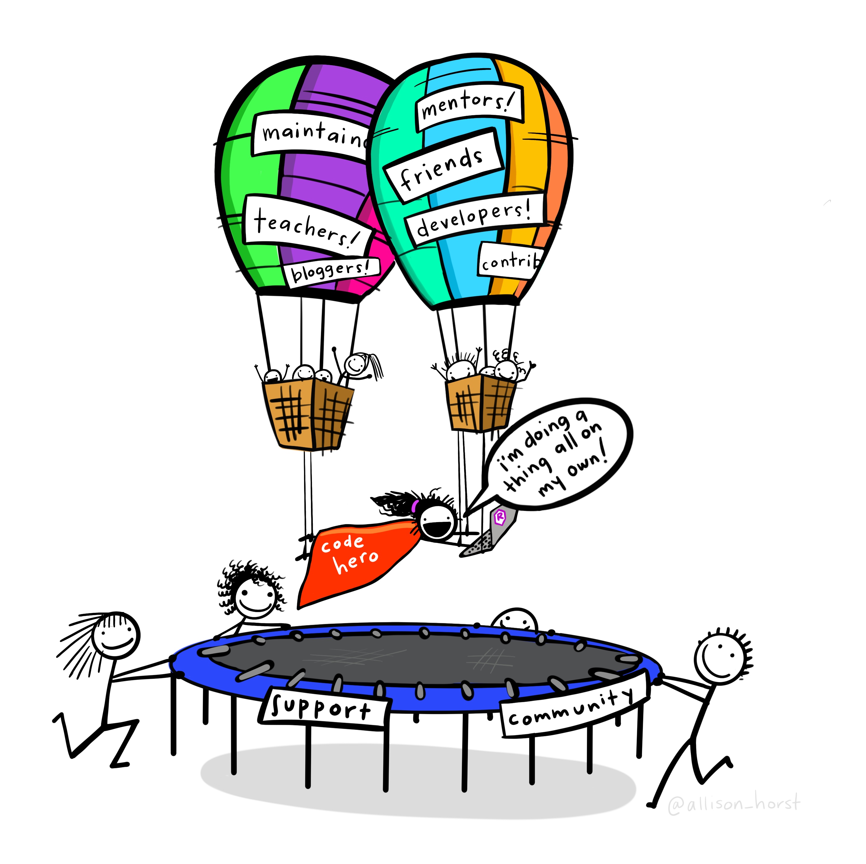
- Each package comes with a website, each of these websites are similarly laid out, and results of example code are displayed, and extensive vignettes describe how to use various functions from the package together

keeping up with the tidyverse
Blog posts highlight updates, along with the reasoning behind them and worked examples
-
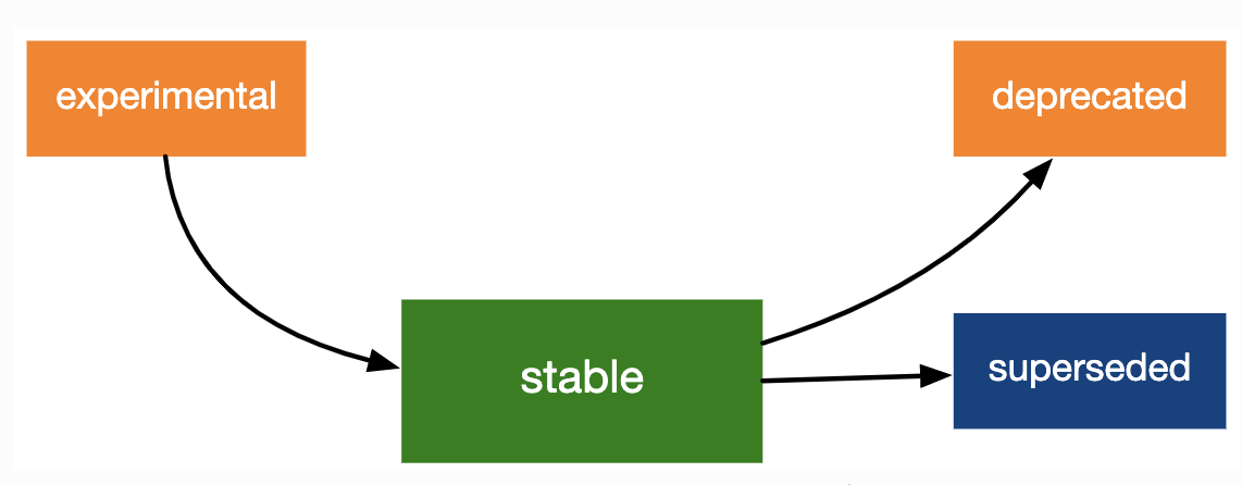
Lifecycle stages and badges
![]()
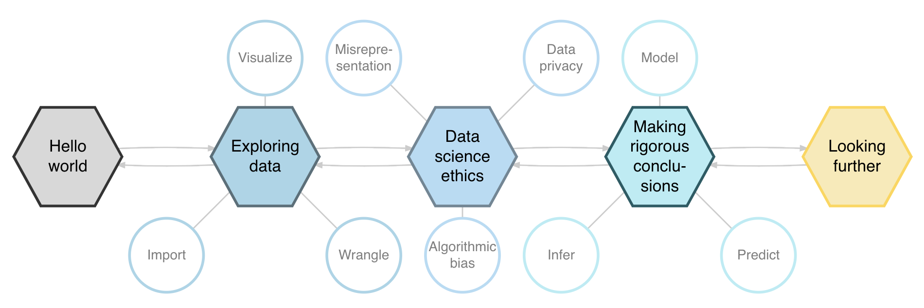
the curriculum we’ve built @ duke statsci
STA 199: Introduction to Data Science
___ the tidyverse
learn the tidyverse
teach the tidyverse