an educator’s perspective of the tidyverse

bit.ly/tidyperspective-pwl

mine çetinkaya-rundel

introduction

collaborators

• Johanna Hardin, Pomona College
• Benjamin S. Baumer, Smith College
• Amelia McNamara, University of St Thomas
• Nicholas J. Horton, Amherst College
• Colin W. Rundel, Duke University

setting the scene

Assumption 1:

Teach authentic tools

Assumption 2:

Teach R as the authentic tool

takeaway

The tidyverse provides an effective and efficient pathway for undergraduate students at all levels and majors to gain computational skills and thinking needed throughout the data science cycle.

Çetinkaya-Rundel, M., Hardin, J., Baumer, B. S., McNamara, A., Horton, N. J., & Rundel, C. (2022). An educator’s perspective of the tidyverse. Technology Innovations in Statistics Education, 14(1). doi.org/10.5070/T514154352.

principles of the tidyverse

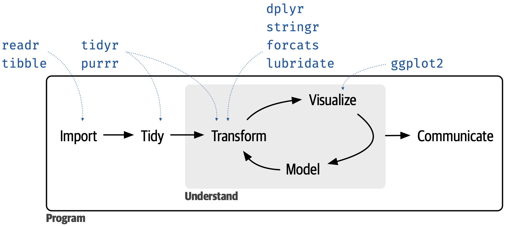
tidyverse

• meta R package that loads eight core packages when invoked and also bundles numerous other packages upon installation
• tidyverse packages share a design philosophy, common grammar, and data structures

setup

Data: Thousands of loans made through the Lending Club, a peer-to-peer lending platform available in the openintro package, with a few modifications.

library(tidyverse)
library(openintro)

loans <- loans_full_schema %>%
  mutate(
    homeownership = str_to_title(homeownership), 
    bankruptcy = if_else(public_record_bankrupt >= 1, "Yes", "No")
  ) %>%
  filter(annual_income >= 10) %>%
  select(
    loan_amount, homeownership, bankruptcy,
    application_type, annual_income, interest_rate
  )

start with a data frame

loans

# A tibble: 9,976 × 6
  loan_amount homeownership bankruptcy application_type annual_income interest…¹
        <int> <chr>         <chr>      <fct>                    <dbl>      <dbl>
1       28000 Mortgage      No         individual               90000      14.1 
2        5000 Rent          Yes        individual               40000      12.6 
3        2000 Rent          No         individual               40000      17.1 
4       21600 Rent          No         individual               30000       6.72
5       23000 Rent          No         joint                    35000      14.1 
6        5000 Own           No         individual               34000       6.72
# … with 9,970 more rows, and abbreviated variable name ¹​interest_rate

tidy data

1. Each variable forms a column
2. Each observation forms a row
3. Each type of observational unit forms a table

Wickham, H. . (2014). Tidy Data. Journal of Statistical Software, 59(10), 1–23. doi.org/10.18637/jss.v059.i10.

task: calculate a summary statistic

Calculate the mean loan amount.

loans

# A tibble: 9,976 × 6
  loan_amount homeownership bankruptcy application_type annual_income interest…¹
        <int> <chr>         <chr>      <fct>                    <dbl>      <dbl>
1       28000 Mortgage      No         individual               90000      14.1 
2        5000 Rent          Yes        individual               40000      12.6 
3        2000 Rent          No         individual               40000      17.1 
4       21600 Rent          No         individual               30000       6.72
5       23000 Rent          No         joint                    35000      14.1 
6        5000 Own           No         individual               34000       6.72
# … with 9,970 more rows, and abbreviated variable name ¹​interest_rate

mean(loan_amount)

Error in mean(loan_amount): object 'loan_amount' not found

accessing a variable

Approach 1: With attach():

attach(loans)
mean(loan_amount)

[1] 16357.53

Not recommended. What if you had another data frame you’re working with concurrently called car_loans that also had a variable called loan_amount in it?

accessing a variable

Approach 2: Using $:

mean(loans$loan_amount)

[1] 16357.53

Approach 3: Using with():

with(loans, mean(loan_amount))

[1] 16357.53

accessing a variable

Approach 4: The tidyverse approach:

loans %>%
  summarise(mean_loan_amount = mean(loan_amount))

# A tibble: 1 × 1
  mean_loan_amount
             <dbl>
1           16358.

• More verbose
• But also more expressive and extensible

the tidyverse approach

• tidyverse functions take a data argument that allows them to localize computations inside the specified data frame

• does not muddy the concept of what is in the current environment: variables always accessed from within in a data frame without the use of an additional function (like with()) or quotation marks, never as a vector

teaching with the tidyverse

task: grouped summary

Based on the applicants’ home ownership status, compute the average loan amount and the number of applicants. Display the results in descending order of average loan amount.

Homeownership	Number of applicants	Average loan amount
Mortgage	$18,132	4,778
Own	$15,665	1,350
Rent	$14,396	3,848

break it down I

Based on the applicants’ home ownership status, compute the average loan amount and the number of applicants. Display the results in descending order of average loan amount.

loans

# A tibble: 9,976 × 6
  loan_amount homeownership bankruptcy application_type annual_income interest…¹
        <int> <chr>         <chr>      <fct>                    <dbl>      <dbl>
1       28000 Mortgage      No         individual               90000      14.1 
2        5000 Rent          Yes        individual               40000      12.6 
3        2000 Rent          No         individual               40000      17.1 
4       21600 Rent          No         individual               30000       6.72
5       23000 Rent          No         joint                    35000      14.1 
6        5000 Own           No         individual               34000       6.72
# … with 9,970 more rows, and abbreviated variable name ¹​interest_rate

break it down II

Based on the applicants’ home ownership status, compute the average loan amount and the number of applicants. Display the results in descending order of average loan amount.

[input] data frame

loans %>%
  group_by(homeownership)

# A tibble: 9,976 × 6
# Groups:   homeownership [3]
  loan_amount homeownership bankruptcy application_type annual_income interest…¹
        <int> <chr>         <chr>      <fct>                    <dbl>      <dbl>
1       28000 Mortgage      No         individual               90000      14.1 
2        5000 Rent          Yes        individual               40000      12.6 
3        2000 Rent          No         individual               40000      17.1 
4       21600 Rent          No         individual               30000       6.72
5       23000 Rent          No         joint                    35000      14.1 
6        5000 Own           No         individual               34000       6.72
# … with 9,970 more rows, and abbreviated variable name ¹​interest_rate

data frame [output]

break it down III

Based on the applicants’ home ownership status, compute the average loan amount and the number of applicants. Display the results in descending order of average loan amount.

loans %>%
  group_by(homeownership) %>% 
  summarize(
    avg_loan_amount = mean(loan_amount)
    )

# A tibble: 3 × 2
  homeownership avg_loan_amount
  <chr>                   <dbl>
1 Mortgage               18132.
2 Own                    15665.
3 Rent                   14396.

break it down IV

Based on the applicants’ home ownership status, compute the average loan amount and the number of applicants. Display the results in descending order of average loan amount.

loans %>%
  group_by(homeownership) %>% 
  summarize(
    avg_loan_amount = mean(loan_amount),
    n_applicants = n()
    )

# A tibble: 3 × 3
  homeownership avg_loan_amount n_applicants
  <chr>                   <dbl>        <int>
1 Mortgage               18132.         4778
2 Own                    15665.         1350
3 Rent                   14396.         3848

break it down V

Based on the applicants’ home ownership status, compute the average loan amount and the number of applicants. Display the results in descending order of average loan amount.

loans %>%
  group_by(homeownership) %>% 
  summarize(
    avg_loan_amount = mean(loan_amount),
    n_applicants = n()
    ) %>%
  arrange(desc(avg_loan_amount))

# A tibble: 3 × 3
  homeownership avg_loan_amount n_applicants
  <chr>                   <dbl>        <int>
1 Mortgage               18132.         4778
2 Own                    15665.         1350
3 Rent                   14396.         3848

putting it back together

[input] data frame

loans %>%
  group_by(homeownership) %>% 
  summarize(
    avg_loan_amount = mean(loan_amount),
    n_applicants = n()
    ) %>%
  arrange(desc(avg_loan_amount))

# A tibble: 3 × 3
  homeownership avg_loan_amount n_applicants
  <chr>                   <dbl>        <int>
1 Mortgage               18132.         4778
2 Own                    15665.         1350
3 Rent                   14396.         3848

[output] data frame

grouped summary with aggregate()

res1 <- aggregate(loan_amount ~ homeownership, 
                  data = loans, FUN = length)
res1

  homeownership loan_amount
1      Mortgage        4778
2           Own        1350
3          Rent        3848

names(res1)[2] <- "n_applicants"
res1

  homeownership n_applicants
1      Mortgage         4778
2           Own         1350
3          Rent         3848

grouped summary with aggregate()

res2 <- aggregate(loan_amount ~ homeownership, 
                  data = loans, FUN = mean)
names(res2)[2] <- "avg_loan_amount"

res2

  homeownership avg_loan_amount
1      Mortgage        18132.45
2           Own        15665.44
3          Rent        14396.44

res <- merge(res1, res2)
res[order(res$avg_loan_amount, decreasing = TRUE), ]

  homeownership n_applicants avg_loan_amount
1      Mortgage         4778        18132.45
2           Own         1350        15665.44
3          Rent         3848        14396.44

grouped summary with aggregate()

res1 <- aggregate(loan_amount ~ homeownership, data = loans, FUN = length)
names(res1)[2] <- "n_applicants"
res2 <- aggregate(loan_amount ~ homeownership, data = loans, FUN = mean)
names(res2)[2] <- "avg_loan_amount"
res <- merge(res1, res2)
res[order(res$avg_loan_amount, decreasing = TRUE), ]

• Good: Inputs and outputs are data frames
• Not so good: Need to introduce

  • formula syntax

  • passing functions as arguments

  • merging datasets

  • square bracket notation for accessing rows

grouped summary with tapply()

sort(
  tapply(loans$loan_amount, loans$homeownership, mean),
  decreasing = TRUE
  )

Mortgage      Own     Rent 
18132.45 15665.44 14396.44 

Not so good:

• passing functions as arguments
• distinguishing between the various apply() functions
• ending up with a new data structure (array)
• reading nested functions

and…

many more comparative examples in the paper

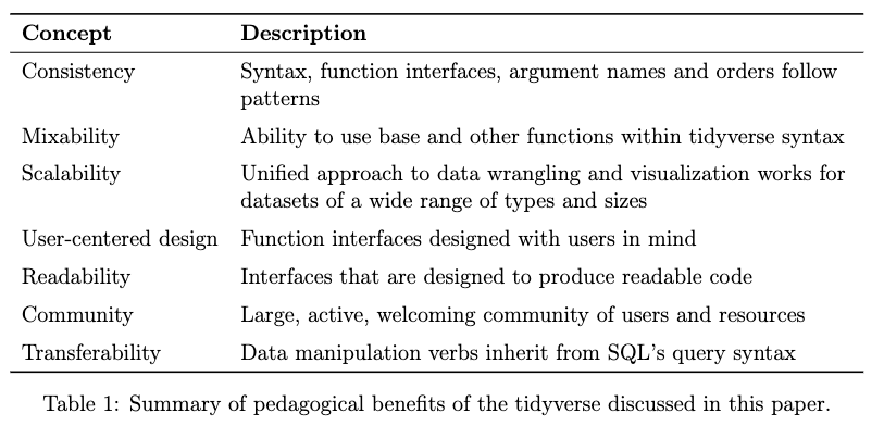
pedagogical strengths of the tidyverse

coda

We are all converts to the tidyverse and have made a conscious choice to use it in our research and our teaching. We each learned R without the tidyverse and have all spent quite a few years teaching without it at a variety of levels from undergraduate introductory statistics courses to graduate statistical computing courses. This paper is a synthesis of the reasons supporting our tidyverse choice, along with benefits and challenges associated with teaching statistics with the tidyverse.

Çetinkaya-Rundel, M., Hardin, J., Baumer, B. S., McNamara, A., Horton, N. J., & Rundel, C. (2022). An educator’s perspective of the tidyverse. Technology Innovations in Statistics Education, 14(1). doi.org/10.5070/T514154352.

thank you!

bit.ly/tidyperspective-pwl