an educator’s perspective of the tidyverse
setting the scene

Assumption 1:
Teach authentic tools

Assumption 2:
Teach R as the authentic tool
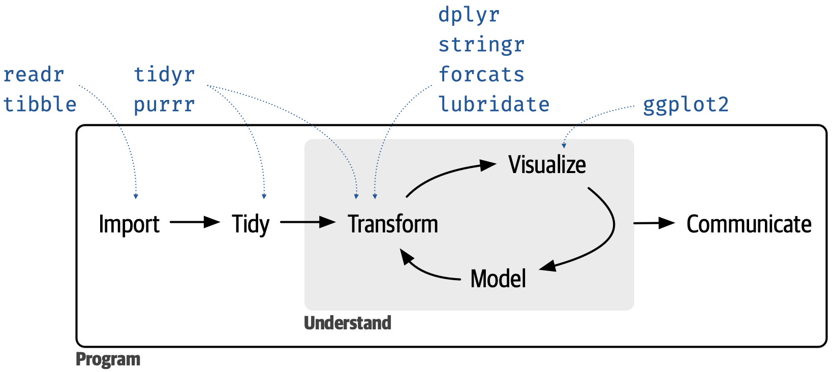
tidyverse
- meta R package that loads eight core packages when invoked and also bundles numerous other packages upon installation
- tidyverse packages share a design philosophy, common grammar, and data structures
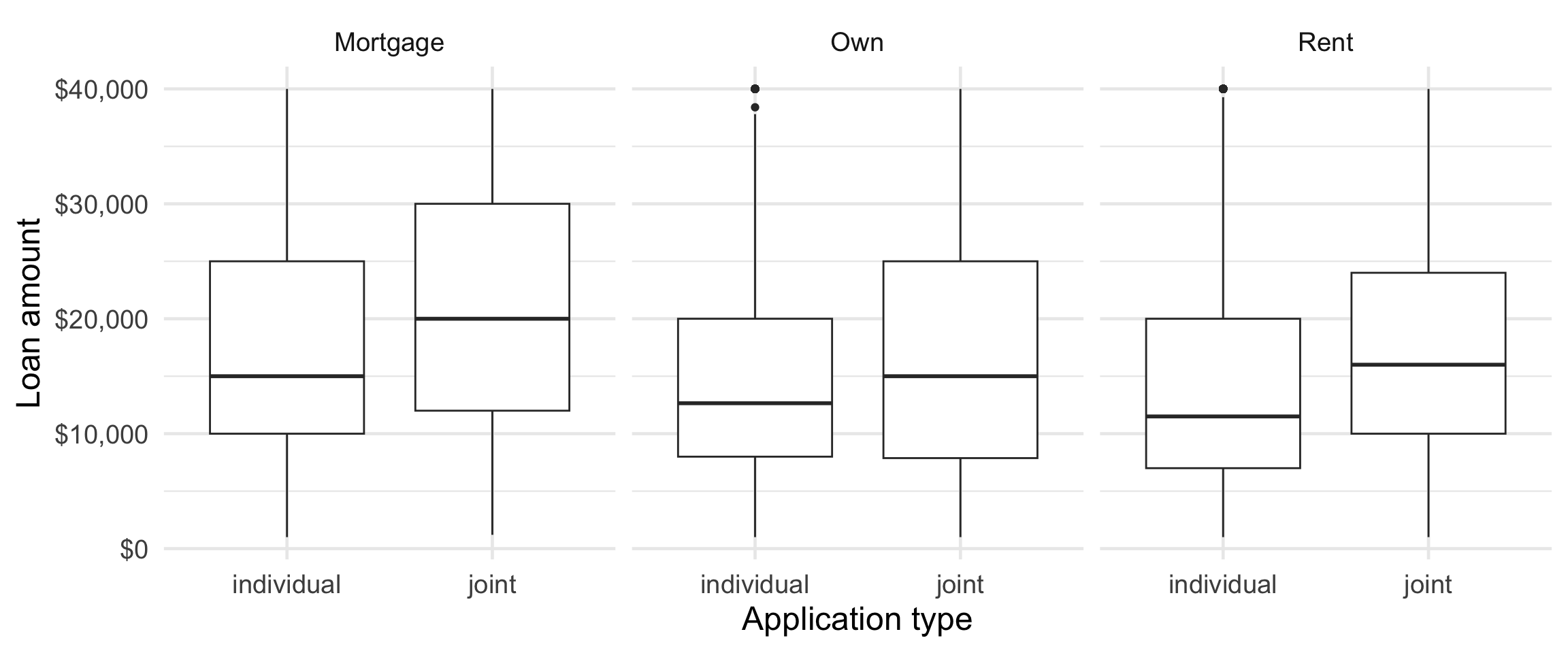
task: data visualization
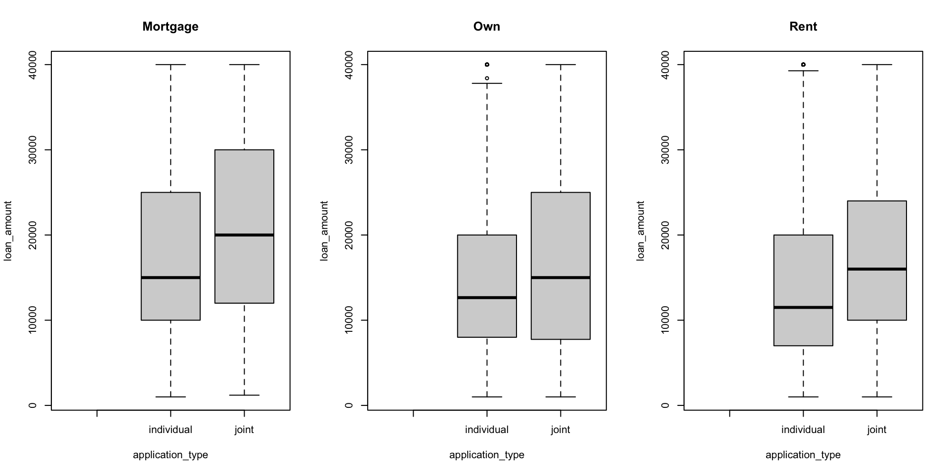
Create side-by-side box plots that shows the relationship between loan amount and application type, faceted by homeownership.
break it down I

break it down II
break it down III
break it down IV
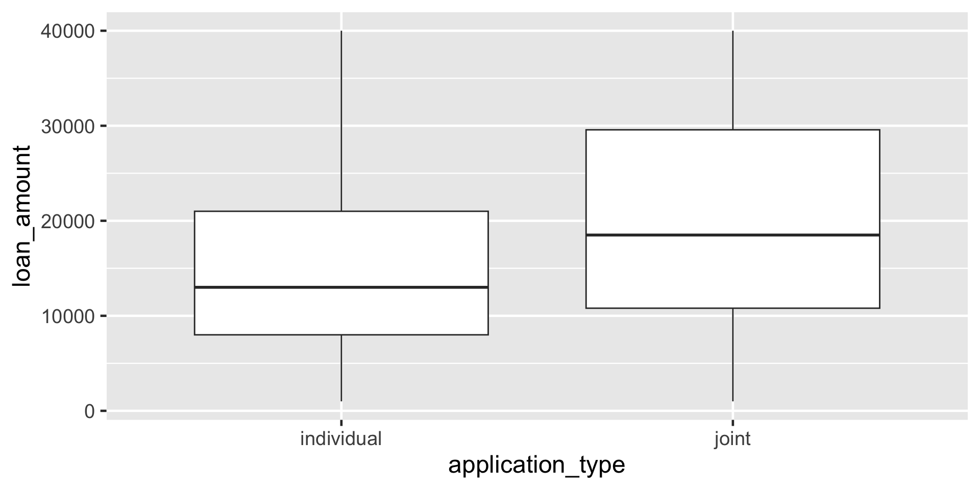
break it down IV
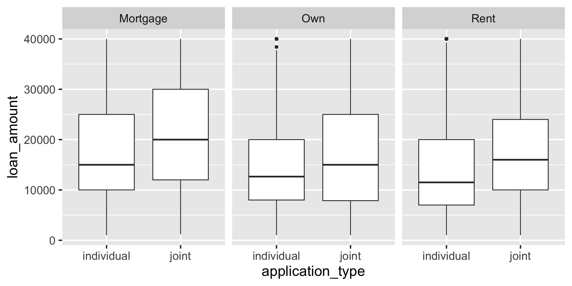
plotting with boxplot()
visualizing a different relationship
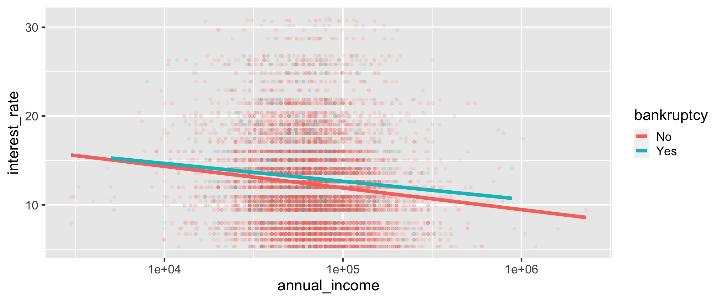
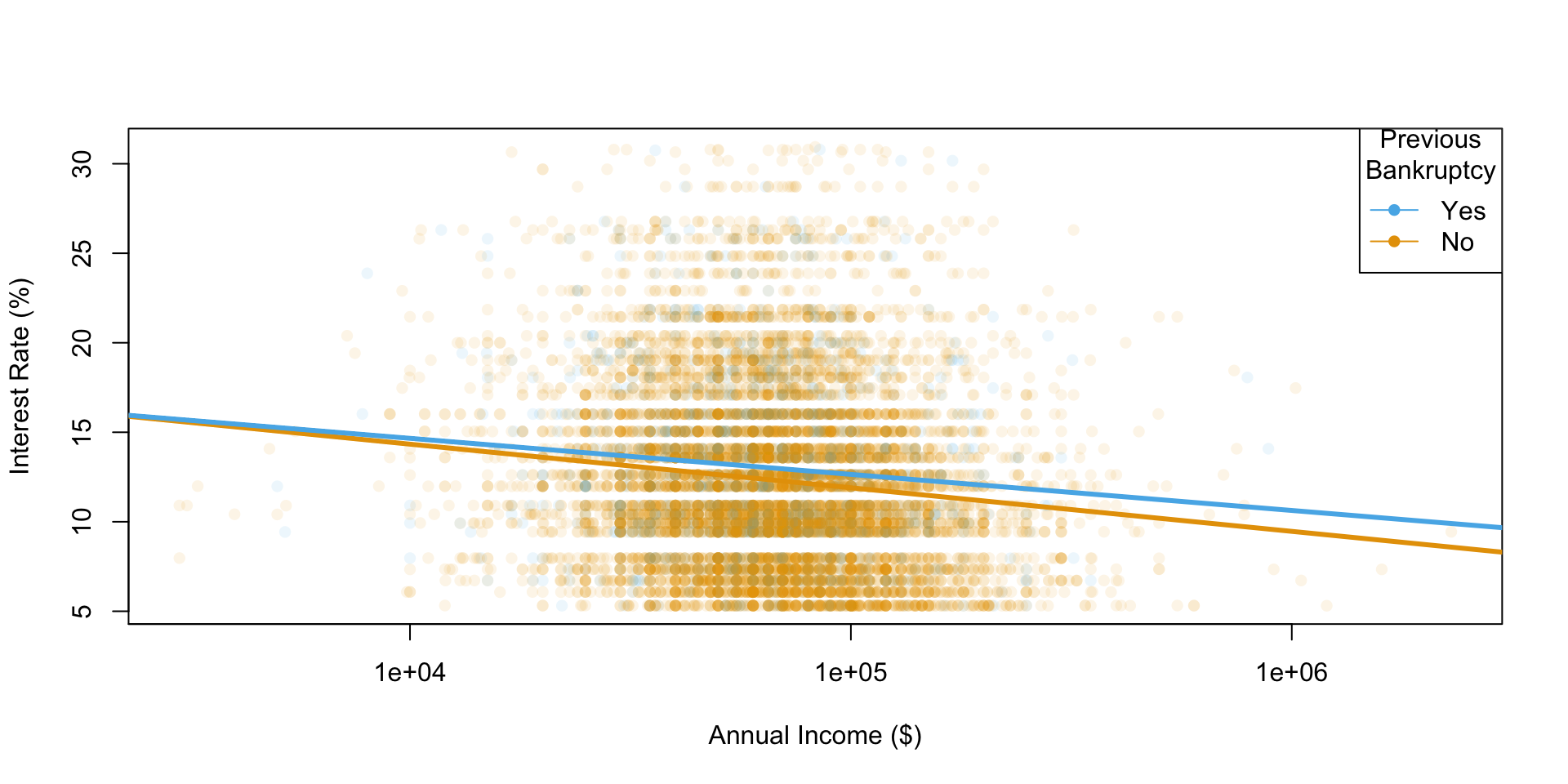
Visualize the relationship between interest rate and annual income, conditioned on whether the applicant had a bankruptcy.
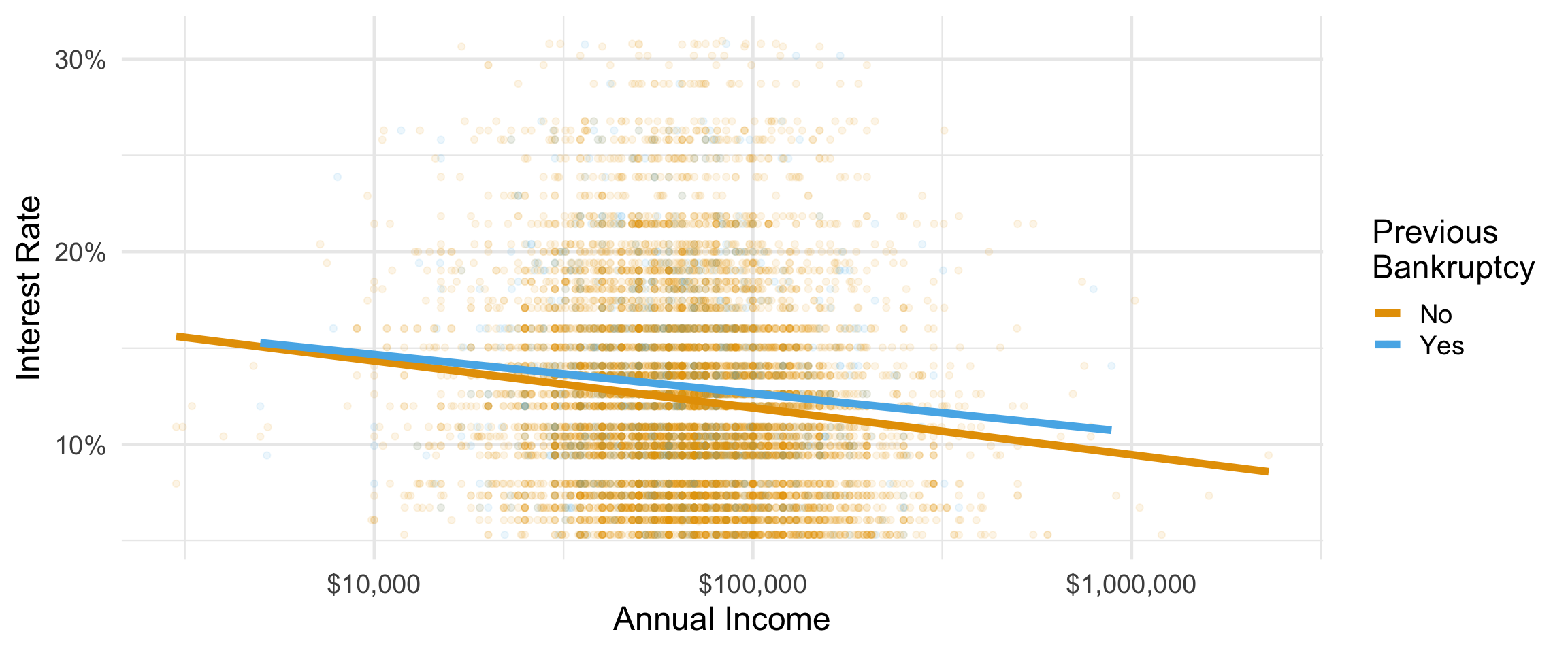
plotting with ggplot()
further customizing ggplot()
ggplot(loans,
       aes(y = interest_rate, x = annual_income,
           color = bankruptcy)) +
  geom_point(alpha = 0.1) +
  geom_smooth(method = "lm", linewidth = 2, se = FALSE) +
  scale_x_log10(labels = scales::label_dollar()) +
  scale_y_continuous(labels = scales::label_percent(scale = 1)) +
  scale_color_OkabeIto() +
  labs(x = "Annual Income", y = "Interest Rate",
       color = "Previous\nBankruptcy") +
  theme_minimal(base_size = 18)
plotting with plot()
keeping up with the tidyverse
Blog posts highlight updates, along with the reasoning behind them and worked examples
-
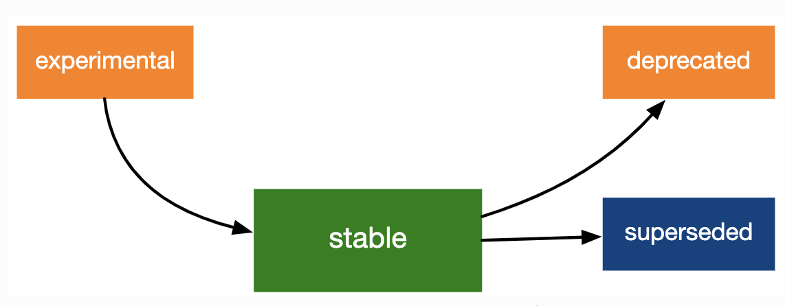
Lifecycle stages and badges
![]()
coda
We are all converts to the tidyverse and have made a conscious choice to use it in our research and our teaching. We each learned R without the tidyverse and have all spent quite a few years teaching without it at a variety of levels from undergraduate introductory statistics courses to graduate statistical computing courses. This paper is a synthesis of the reasons supporting our tidyverse choice, along with benefits and challenges associated with teaching statistics with the tidyverse.