class: center, middle, inverse, title-slide # Building multivariate visualizations <br> with ggplot2 ## Max Planck School of Cognition ### Dr. Mine Çetinkaya-Rundel ### 6 Jan 2020 <br><br> <a href="bit.ly/ggplot2-mpc">http://bit.ly/ggplot2-mpc</a> --- class: center, middle # Data visualization --- ## Data visualization > *"The simple graph has brought more information to the data analyst’s mind than any other device." > — John Tukey* - Data visualization is the creation and study of the visual representation of data. - Many tools for visualizing data (R is one of them) - Many approaches/systems within R for making data visualizations, **ggplot2** is one of them --- ## ggplot2 `\(\in\)` tidyverse .pull-left[ <img src="img/ggplot2-part-of-tidyverse.png" width="80%" /> ] .pull-right[ - **ggplot2**: tidyverse's data visualization package - `gg` in "ggplot2" stands for Grammar of Graphics - Inspired by the book **Grammar of Graphics** by Leland Wilkinson - A grammar of graphics is a tool that enables concise description of components of a graphic <img src="img/grammar-of-graphics.png" width="80%" /> ] --- ## Following along... .pull-left[ ### Option 1: RStudio local - Download the materials at [http://bit.ly/ggplot2-mpc](bit.ly/ggplot2-mpc)" and launch `ggplot2-max-planck.Rproj` - Install and load `tidyverse` and `ggrepel` ```r install.packages("tidyverse") install.packages("ggrepel") library(tidyverse) library(ggrepel) ``` - Open `exercises.Rmd` ] .pull-right[ ### Option 2: RStudio Cloud - Open the RStudio Cloud project at http://bit.ly/2umsmNT - Open the R Markdown file in the project called `exercises.Rmd` ] --- ## Datasets * Transit ride data + `daily`: daily summary of rides ```r daily <- read_csv("data/daily.csv") ``` * Durham registered voter data + `durham_voters`: one row per voter ```r durham_voters <- read_csv("data/durham_voters.csv") ``` --- class: center, middle # Layer up! --- <!-- --> --- **Warm up:** Which of the two datasets does this visualization use? Determine which variable is mapped to which aesthetic (x-axis, y-axis, etc.) element of the dataset. <!-- --> --- ## ggplot2 template Make any plot by filling in the parameters of this template <img src="img/ggplot2-template.png" width="100%" /> --- ```r ggplot(data = daily) ``` <!-- --> --- ```r ggplot(data = daily, mapping = aes(x = ride_date, y = n_rides)) ``` <!-- --> --- ```r ggplot(data = daily, mapping = aes(x = ride_date, y = n_rides)) + geom_point() ``` <!-- --> --- ```r ggplot(data = daily, aes(x = ride_date, y = n_rides, color = day_of_week)) + geom_point() ``` <!-- --> --- ```r ggplot(data = daily, aes(x = ride_date, y = n_rides, color = day_of_week)) + geom_smooth() ``` ``` ## `geom_smooth()` using method = 'loess' and formula 'y ~ x' ``` <!-- --> --- ```r ggplot(data = daily, aes(x = ride_date, y = n_rides, color = day_of_week)) + geom_smooth(method = "loess") ``` <!-- --> --- ```r ggplot(data = daily, aes(x = ride_date, y = n_rides, color = day_of_week)) + geom_smooth(method = "loess", se = FALSE) ``` <!-- --> --- ```r ggplot(data = daily, aes(x = ride_date, y = n_rides, color = day_of_week)) + geom_smooth(method = "loess", se = FALSE) + scale_color_viridis_d() ``` 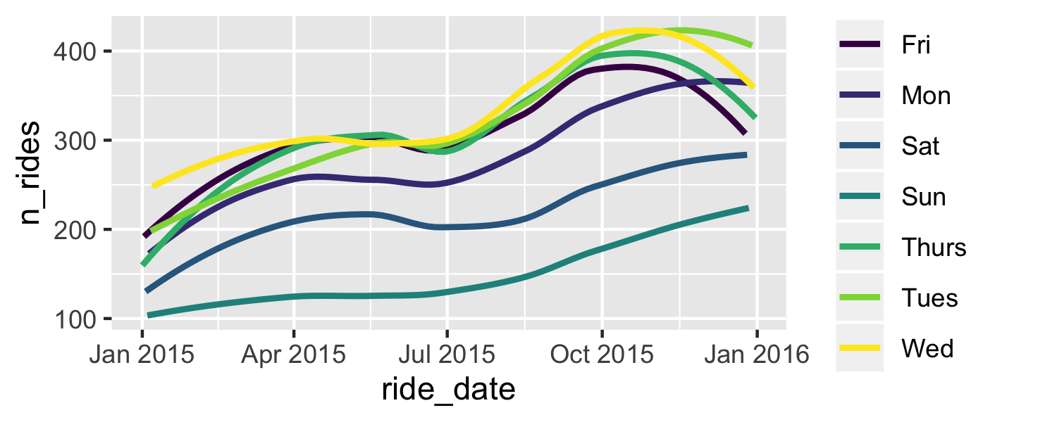<!-- --> --- ```r ggplot(data = daily, aes(x = ride_date, y = n_rides, color = day_of_week)) + geom_smooth(method = "loess", se = FALSE) + scale_color_viridis_d() + theme_minimal() ``` <!-- --> --- ```r ggplot(data = daily, aes(x = ride_date, y = n_rides, color = day_of_week)) + geom_smooth(method = "loess", se = FALSE) + scale_color_viridis_d() + theme_minimal() + labs(x = "Ride date", y = "Number of rides", color = "Day of week", title = "Daily rides", subtitle = "Durham, NC") ``` <!-- --> --- ```r daily <- daily %>% mutate(day_of_week = fct_relevel(day_of_week, "Mon", "Tues", "Wed", "Thurs", "Fri", "Sat", "Sun")) ggplot(data = daily, aes(x = ride_date, y = n_rides, color = day_of_week)) + geom_smooth(se = FALSE, method = "loess") + scale_color_viridis_d() + theme_minimal() + labs(x = "Ride date", y = "Number of rides", color = "Day of week", title = "Daily rides", subtitle = "Durham, NC") ``` --- <!-- --> --- ## ggplot, the making of 1. "Initialize" a plot with ggplot() 2. Add layers with geom_ functions ``` ggplot(data = <DATA>) + <GEOM_FUNCTION>(mapping = aes(<MAPPINGS>))+ geom_point(mapping = aes(x = displ, y = hwy)) ``` --- class: center, middle # Mapping --- ## Size by number of riders ```r ggplot(data = daily, aes(x = ride_date, y = n_rides, size = n_riders)) + geom_point() ``` <!-- --> --- ## Set alpha value ```r ggplot(data = daily, aes(x = ride_date, y = n_rides, size = n_riders)) + geom_point(alpha = 0.5) ``` <!-- --> --- **Exercise 1:** Using information from https://ggplot2.tidyverse.org/articles/ggplot2-specs.html add `color`, `size`, `alpha`, and `shape` aesthetics to your graph. Experiment. Do different things happen when you map aesthetics to discrete and continuous variables? What happens when you use more than one aesthetic? ```r ggplot(data = daily, aes(x = ride_date, y = n_rides, color = day_of_week)) + geom_smooth(method = "loess", se = FALSE) + scale_color_viridis_d() + theme_minimal() + labs(x = "Ride date", y = "Number of rides", color = "Day of week", title = "Daily rides", subtitle = "Durham, NC") ``` ```r names(daily) ``` ``` ## [1] "ride_date" "day_of_week" "month" "n_rides" ## [5] "n_riders" "n_unique_stops" "n_unique_routes" ``` --- <img src="img/aesthetic-mappings.png" width="80%" /> --- ## Mappings can be at the `geom` level ```r ggplot(data = daily) + geom_point(mapping = aes(x = ride_date, y = n_rides)) ``` <!-- --> --- ## Different mappings for different `geom`s ```r ggplot(data = daily, mapping = aes(x = ride_date, y = n_rides)) + geom_point() + geom_smooth(aes(color = day_of_week), method = "loess", se = FALSE) ``` <!-- --> --- ## Set vs. map .pull-left[ To **map** an aesthetic to a variable, place it inside `aes()` ```r ggplot(data = daily, mapping = aes(x = ride_date, y = n_rides, color = day_of_week)) + geom_point() ``` <!-- --> ] .pull-right[ To **set** an aesthetic to a value, place it outside `aes()` ```r ggplot(data = daily, mapping = aes(x = ride_date, y = n_rides)) + geom_point(color = "red") ``` 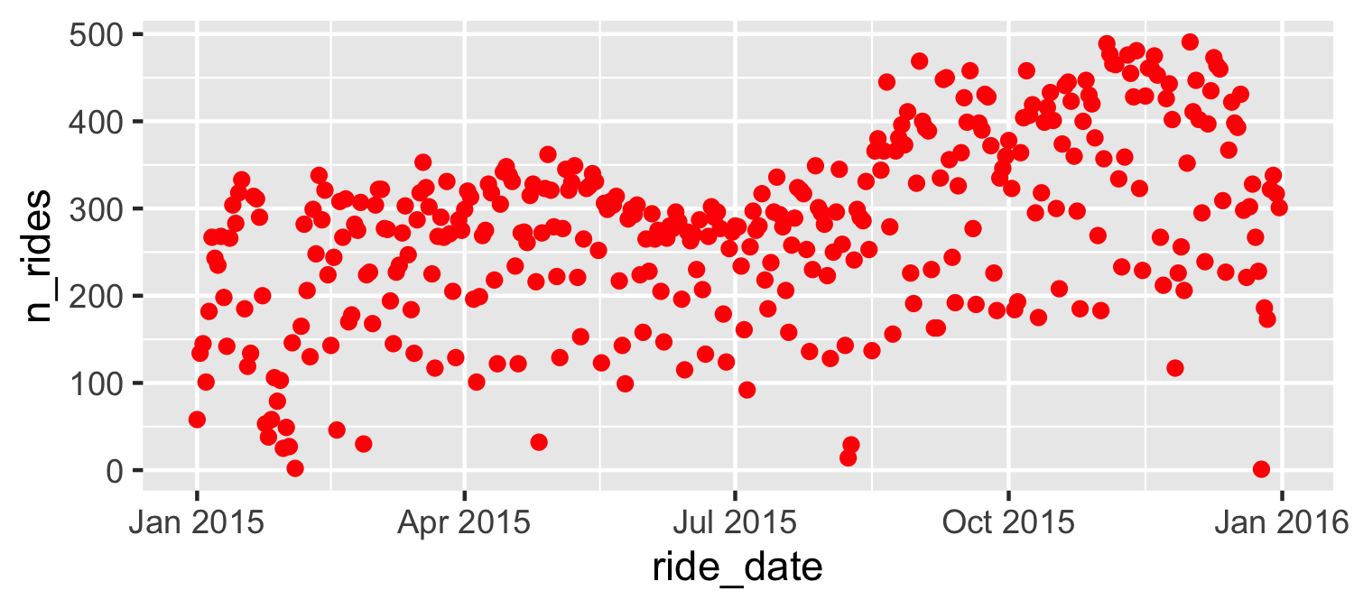<!-- --> ] --- class: center, middle # Syntax --- ## Data can be passed in ```r daily %>% ggplot(aes(x = ride_date, y = n_rides)) + geom_point() ``` <!-- --> --- ## Parameters can be unnamed ```r ggplot(daily, aes(x = ride_date, y = n_rides)) + geom_point() ``` <!-- --> --- ## Variable creation on the fly... Color by weekday / weekend ```r ggplot(data = daily, aes(x = ride_date, y = n_rides, color = day_of_week %in% c("Sat", "Sun"))) + geom_point() ``` 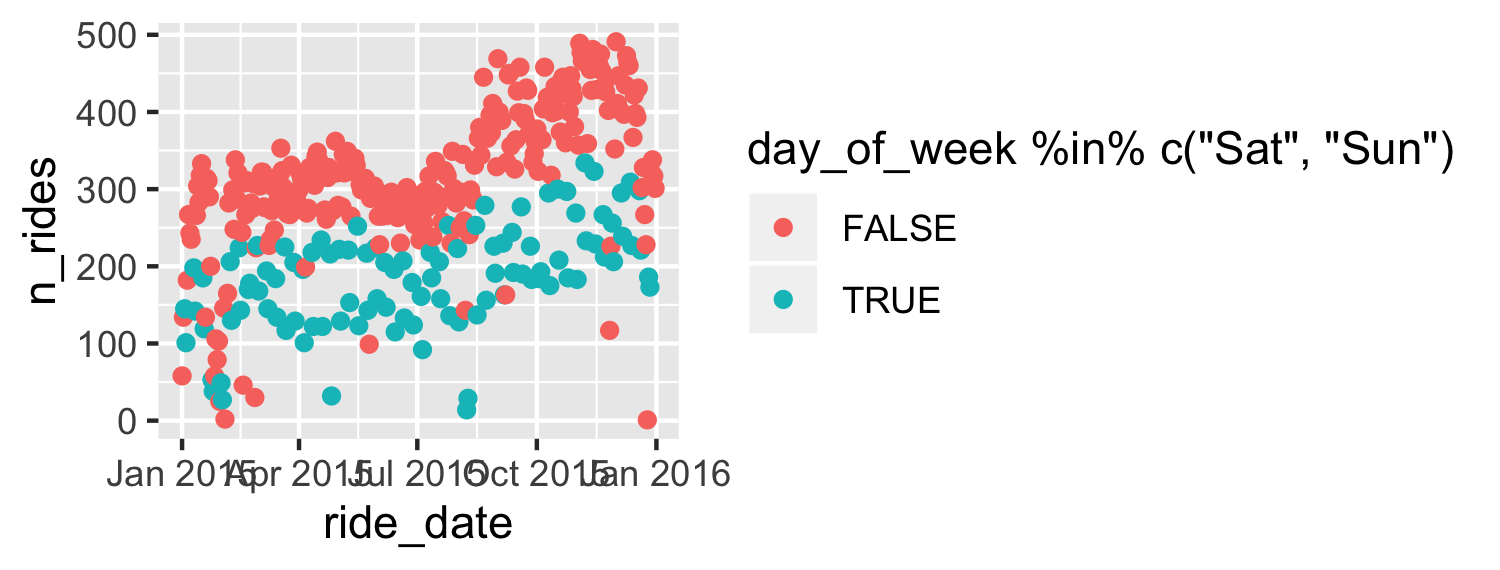<!-- --> --- ## Variable creation on the fly... ```r ggplot(data = daily, aes(x = ride_date, y = n_rides, color = day_of_week %in% c("Sat", "Sun"))) + geom_point() + labs(color = "Weekend") ``` 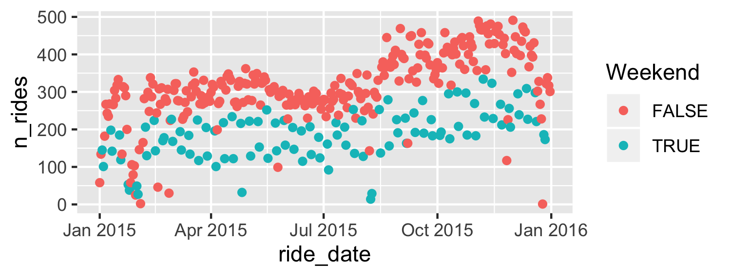<!-- --> --- ## ... or passed in ```r daily %>% mutate(day_type = if_else(day_of_week %in% c("Sat", "Sun"), "Weekend", "Weekday")) %>% ggplot(aes(x = ride_date, y = n_rides, color = day_type)) + geom_point() ``` 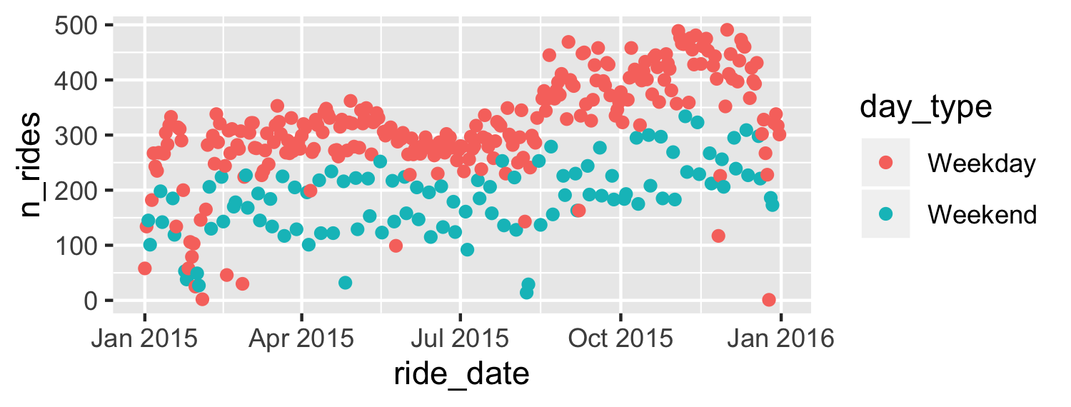<!-- --> --- class: center, middle # Common early pitfalls --- ## Mappings that aren't ```r ggplot(data = daily) + geom_point(aes(x = ride_date, y = n_rides, color = "blue")) ``` <!-- --> --- ## Mappings that aren't ```r ggplot(data = daily) + geom_point(aes(x = ride_date, y = n_rides), color = "blue") ``` 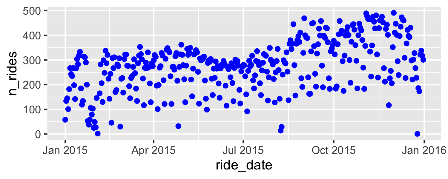<!-- --> --- ## + and %>% **Exercise 2:** What is wrong with the following? ```r daily %>% mutate(day_type = if_else(day_of_week %in% c("Sat", "Sun"), "Weekend", "Weekday")) %>% ggplot(aes(x = ride_date, y = n_rides, color = day_type)) %>% geom_point() ``` --- ## + and %>% What is wrong with the following? ```r daily %>% mutate(day_type = if_else(day_of_week %in% c("Sat", "Sun"), "Weekend", "Weekday")) %>% ggplot(aes(x = ride_date, y = n_rides, color = day_type)) %>% geom_point() ``` ``` ## Error: `mapping` must be created by `aes()` ## Did you use %>% instead of +? ``` --- class: center, middle # Building up layer by layer --- ## Basic plot ```r ggplot(data = daily, aes(x = ride_date, y = n_rides)) + geom_point() ``` <!-- --> --- ## Two layers! ```r ggplot(data = daily, aes(x = ride_date, y = n_rides)) + geom_point() + geom_line() ``` <!-- --> --- ## Iterate on layers ```r ggplot(data = daily, aes(x = ride_date, y = n_rides)) + geom_point() + geom_smooth(span = 0.1) # try changing span ``` ``` ## `geom_smooth()` using method = 'loess' and formula 'y ~ x' ``` <!-- --> --- ## The power of groups ```r ggplot(data = daily, aes(x = ride_date, y = n_rides, color = day_of_week)) + geom_point() + geom_line() ``` 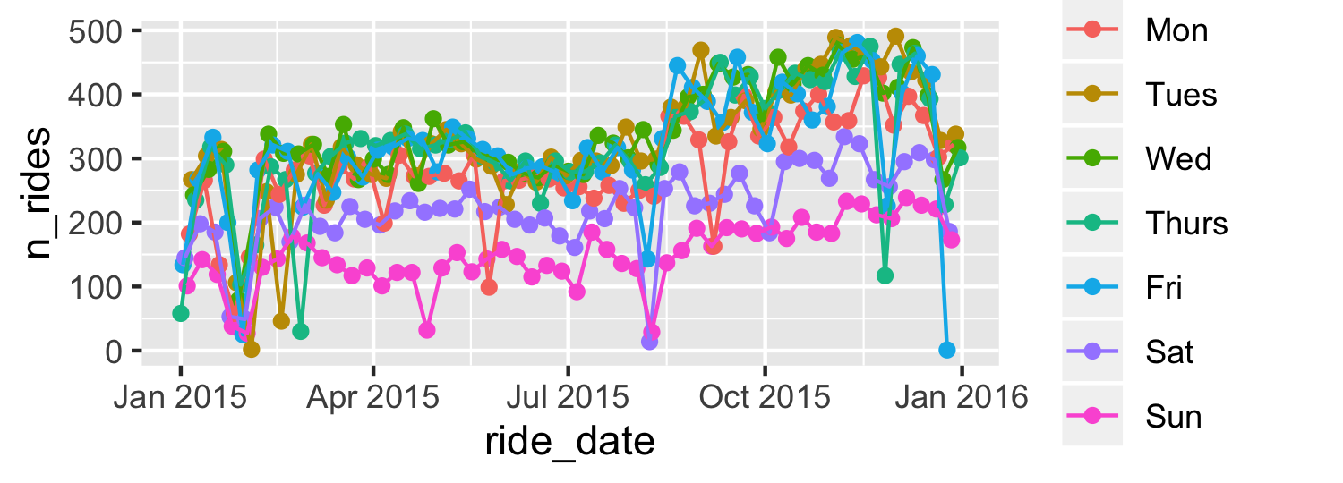<!-- --> --- ## Now we've got it ```r ggplot(data = daily, aes(x = ride_date, y = n_rides, color = day_of_week)) + geom_smooth(span = 0.2, se = FALSE) ``` ``` ## `geom_smooth()` using method = 'loess' and formula 'y ~ x' ``` 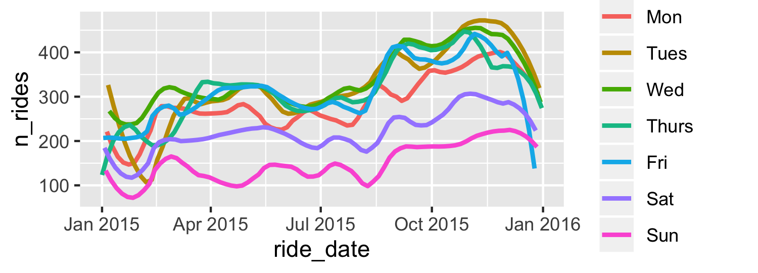<!-- --> --- ## Control data by layer ```r ggplot(data = daily, aes(x = ride_date, y = n_rides, color = day_of_week)) + geom_point(data = filter(daily, !(day_of_week %in% c("Sat", "Sun")) & n_rides < 200), size = 5, color = "gray") + geom_point() ``` <!-- --> --- **Exercise 3:** Work with your neighbor to sketch what the following plot will look like. No cheating! Do not run the code, just think through the code for the time being. ```r low_weekdays <- daily %>% filter(!(day_of_week %in% c("Sat", "Sun")) & n_rides < 100) ggplot(daily, aes(x = ride_date, y = n_rides, color = day_of_week)) + geom_point(data = low_weekdays, size = 5, color = "gray") + geom_point() + geom_text(data = low_weekdays, aes(y = n_rides + 15, label = ride_date), size = 2, color = "black") ``` --- ```r low_weekdays <- daily %>% filter(!(day_of_week %in% c("Sat", "Sun")) & n_rides < 100) low_weekdays ``` ``` ## # A tibble: 9 x 7 ## ride_date day_of_week month n_rides n_riders n_unique_stops ## <date> <fct> <chr> <dbl> <dbl> <dbl> ## 1 2015-01-01 Thurs Jan 58 37 44 ## 2 2015-01-26 Mon Jan 58 52 15 ## 3 2015-01-28 Wed Jan 79 65 11 ## 4 2015-01-30 Fri Jan 25 25 12 ## 5 2015-02-03 Tues Feb 2 2 2 ## 6 2015-02-17 Tues Feb 46 34 33 ## 7 2015-02-26 Thurs Feb 30 22 22 ## 8 2015-05-25 Mon May 99 55 66 ## 9 2015-12-25 Fri Dec 1 1 1 ## # … with 1 more variable: n_unique_routes <dbl> ``` --- ```r ggplot(daily, aes(x = ride_date, y = n_rides, color = day_of_week)) + geom_point() ``` <!-- --> --- ```r ggplot(daily, aes(x = ride_date, y = n_rides, color = day_of_week)) + geom_point() + geom_point(data = low_weekdays, size = 5, color = "gray") ``` <!-- --> --- ```r ggplot(daily, aes(x = ride_date, y = n_rides, color = day_of_week)) + geom_point(data = low_weekdays, size = 5, color = "gray") + geom_point() ``` <!-- --> --- ```r ggplot(daily, aes(x = ride_date, y = n_rides, color = day_of_week)) + geom_point(data = low_weekdays, size = 5, color = "gray") + geom_point() + geom_text(data = low_weekdays, aes(y = n_rides, label = ride_date), size = 2, color = "black") ``` <!-- --> --- ```r ggplot(daily, aes(x = ride_date, y = n_rides, color = day_of_week)) + geom_point(data = low_weekdays, size = 5, color = "gray") + geom_point() + geom_text(data = low_weekdays, aes(y = n_rides + 15, label = ride_date), size = 2, color = "black") ``` <!-- --> --- ```r library(ggrepel) ggplot(daily, aes(x = ride_date, y = n_rides, color = day_of_week)) + geom_point(data = low_weekdays, size = 5, color = "gray") + geom_point() + geom_text_repel(data = low_weekdays, aes(x = ride_date, y = n_rides, label = as.character(ride_date)), size = 3, color = "black") ``` 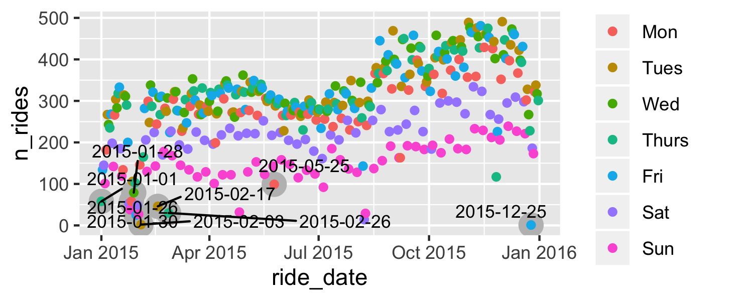<!-- --> --- ```r ggplot(daily, aes(x = ride_date, y = n_rides, color = day_of_week)) + geom_point(data = low_weekdays, size = 5, color = "gray") + geom_point() + geom_label_repel(data = low_weekdays, aes(x = ride_date, y = n_rides, label = as.character(ride_date)), size = 2, color = "black") ``` <!-- --> --- **Exercise 4:** How would you fix the following plot to color by day of week? ```r ggplot(daily, aes(x = ride_date, y = n_rides, color = day_of_week)) + geom_smooth(color = "blue") ``` ``` ## `geom_smooth()` using method = 'loess' and formula 'y ~ x' ``` 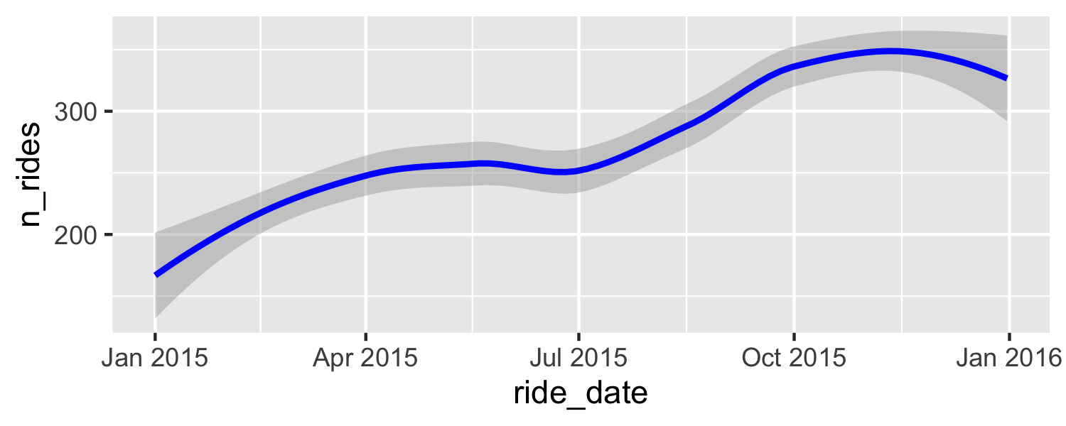<!-- --> --- ## Other geoms - There are a number of other geoms besides `geom_point()`, `geom_line()`, `geom_smooth()`, and `geom_text()`. - More info: [ggplot2.tidyverse.org/reference](https://ggplot2.tidyverse.org/reference/) --- class: center, middle # Splitting over facets --- ## Data prep ```r daily <- daily %>% mutate( day = if_else(day_of_week %in% c("Sat", "Sun"), "Weekend", "Weekday"), temp = if_else(month %in% c("Jan", "Feb", "Mar", "Dec", "Nov", "Oct"), "Cooler", "Warmer") ) %>% select(day, temp, everything()) daily ``` ``` ## # A tibble: 364 x 9 ## day temp ride_date day_of_week month n_rides n_riders n_unique_stops ## <chr> <chr> <date> <fct> <chr> <dbl> <dbl> <dbl> ## 1 Week… Cool… 2015-01-01 Thurs Jan 58 37 44 ## 2 Week… Cool… 2015-01-02 Fri Jan 134 83 93 ## 3 Week… Cool… 2015-01-03 Sat Jan 145 84 100 ## 4 Week… Cool… 2015-01-04 Sun Jan 101 57 63 ## 5 Week… Cool… 2015-01-05 Mon Jan 182 117 109 ## 6 Week… Cool… 2015-01-06 Tues Jan 267 138 146 ## 7 Week… Cool… 2015-01-07 Wed Jan 243 157 129 ## 8 Week… Cool… 2015-01-08 Thurs Jan 235 154 141 ## 9 Week… Cool… 2015-01-09 Fri Jan 268 173 147 ## 10 Week… Cool… 2015-01-10 Sat Jan 198 114 116 ## # … with 354 more rows, and 1 more variable: n_unique_routes <dbl> ``` --- ## facet_wrap ```r ggplot(data = daily, aes(x = ride_date, y = n_rides)) + geom_line() + facet_wrap( ~ day) ``` 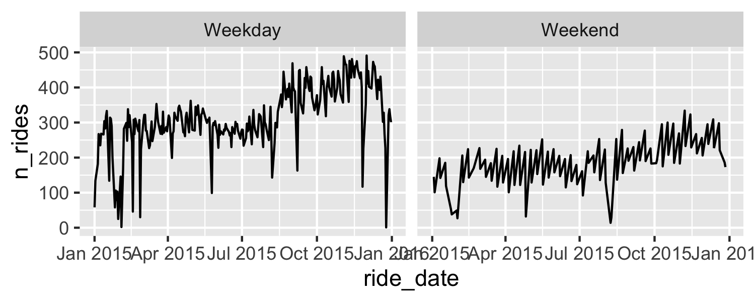<!-- --> --- ## facet_grid ```r ggplot(data = daily, aes(x = ride_date, y = n_rides)) + geom_line() + facet_grid(temp ~ day) ``` <!-- --> --- ## facet_grid ```r ggplot(data = daily, aes(x = ride_date, y = n_rides)) + geom_line() + facet_grid(day ~ temp) ``` 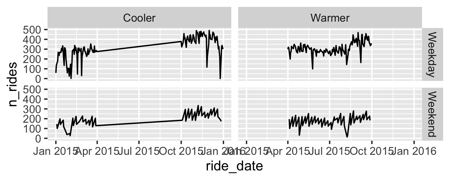<!-- --> --- ## Durham voters ```r durham_voters %>% select(race_code, gender_code, age) ``` ``` ## # A tibble: 204,063 x 3 ## race_code gender_code age ## <chr> <chr> <chr> ## 1 I M Age Over 66 ## 2 U U Age 18 - 25 ## 3 O F Age 41 - 65 ## 4 W F Age 41 - 65 ## 5 W M Age 41 - 65 ## 6 B M Age 26 - 40 ## 7 W F Age 41 - 65 ## 8 W M Age 26 - 40 ## 9 B F Age 41 - 65 ## 10 B M Age 41 - 65 ## # … with 204,053 more rows ``` --- ## Data prep ```r durham_voters %>% group_by(race_code, gender_code, age) %>% summarize(n_voters = n(), n_rep = sum(party == "REP")) ``` ``` ## # A tibble: 92 x 5 ## # Groups: race_code, gender_code [21] ## race_code gender_code age n_voters n_rep ## <chr> <chr> <chr> <int> <int> ## 1 A F Age < 18 Or Invalid Birth Date 2 0 ## 2 A F Age 18 - 25 751 35 ## 3 A F Age 26 - 40 1086 64 ## 4 A F Age 41 - 65 727 75 ## 5 A F Age Over 66 170 36 ## 6 A M Age 18 - 25 635 42 ## 7 A M Age 26 - 40 919 64 ## 8 A M Age 41 - 65 572 61 ## 9 A M Age Over 66 175 33 ## 10 A U Age 18 - 25 8 1 ## # … with 82 more rows ``` --- ## Data prep ```r durham_voters_summary <- durham_voters %>% group_by(race_code, gender_code, age) %>% summarize(n_all_voters = n(), n_rep_voters = sum(party == "REP")) %>% filter(gender_code %in% c("F", "M") & race_code %in% c("W", "B", "A") & age != "Age < 18 Or Invalid Birth Date") durham_voters_summary ``` ``` ## # A tibble: 24 x 5 ## # Groups: race_code, gender_code [6] ## race_code gender_code age n_all_voters n_rep_voters ## <chr> <chr> <chr> <int> <int> ## 1 A F Age 18 - 25 751 35 ## 2 A F Age 26 - 40 1086 64 ## 3 A F Age 41 - 65 727 75 ## 4 A F Age Over 66 170 36 ## 5 A M Age 18 - 25 635 42 ## 6 A M Age 26 - 40 919 64 ## 7 A M Age 41 - 65 572 61 ## 8 A M Age Over 66 175 33 ## 9 B F Age 18 - 25 7446 133 ## 10 B F Age 26 - 40 13686 203 ## # … with 14 more rows ``` --- ## facet_grid ```r ggplot(durham_voters_summary, aes(x = age, y = n_all_voters)) + geom_bar(stat = "identity") + facet_grid(race_code ~ gender_code) ``` <!-- --> --- ## Free scales ```r ggplot(durham_voters_summary, aes(x = age, y = n_all_voters)) + geom_bar(stat = "identity") + facet_grid(race_code ~ gender_code, scales = "free_y") ``` <!-- --> --- **Exercise 5:** In what ways is the following plot different than the previous? 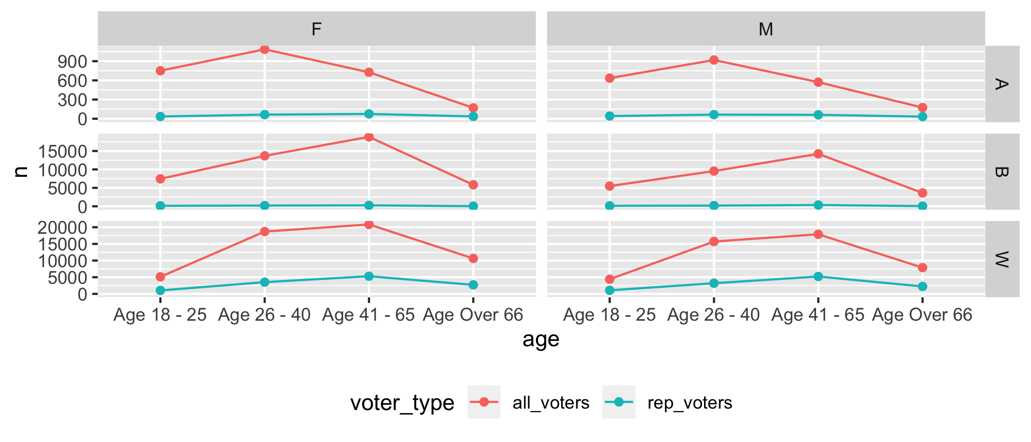<!-- --> --- ```r durham_voters_summary ``` ``` ## # A tibble: 24 x 5 ## # Groups: race_code, gender_code [6] ## race_code gender_code age n_all_voters n_rep_voters ## <chr> <chr> <chr> <int> <int> ## 1 A F Age 18 - 25 751 35 ## 2 A F Age 26 - 40 1086 64 ## 3 A F Age 41 - 65 727 75 ## 4 A F Age Over 66 170 36 ## 5 A M Age 18 - 25 635 42 ## 6 A M Age 26 - 40 919 64 ## 7 A M Age 41 - 65 572 61 ## 8 A M Age Over 66 175 33 ## 9 B F Age 18 - 25 7446 133 ## 10 B F Age 26 - 40 13686 203 ## # … with 14 more rows ``` --- class: center, middle <img src="img/pivot.gif" width="80%" style="display: block; margin: auto;" /> --- ## `pivot_*()` functions 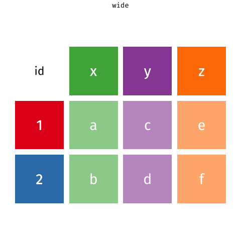<!-- --> --- ## `pivot_longer()` ```r pivot_longer(data, cols, names_to = "name", values_to = "value") ``` - The first argument is `data` as usual. - The second argument, `cols`, is where you specify which columns to pivot into longer format -- in this case any column starting with `n`: `starts_with("n_")` - The third argument, `names_to`, is a string specifying the name of the column to create from the data stored in the column names of data -- in this case `voter_type` - The fourth argument, `values_to`, is a string specifying the name of the column to create from the data stored in cell values, in this case `n` - We'll also prefix these names with `n` --- ```r durham_voters_summary %>% tidyr::pivot_longer(cols = starts_with("n_"), names_to = "voter_type", values_to = "n", names_prefix = "n_") ``` ``` ## # A tibble: 48 x 5 ## # Groups: race_code, gender_code [6] ## race_code gender_code age voter_type n ## <chr> <chr> <chr> <chr> <int> ## 1 A F Age 18 - 25 all_voters 751 ## 2 A F Age 18 - 25 rep_voters 35 ## 3 A F Age 26 - 40 all_voters 1086 ## 4 A F Age 26 - 40 rep_voters 64 ## 5 A F Age 41 - 65 all_voters 727 ## 6 A F Age 41 - 65 rep_voters 75 ## 7 A F Age Over 66 all_voters 170 ## 8 A F Age Over 66 rep_voters 36 ## 9 A M Age 18 - 25 all_voters 635 ## 10 A M Age 18 - 25 rep_voters 42 ## # … with 38 more rows ``` --- ## Facets + layers ```r durham_voters_summary %>% pivot_longer(cols = starts_with("n_"), names_to = "voter_type", values_to = "n", names_prefix = "n_") %>% mutate(age_cat = as.numeric(as.factor(age))) %>% ggplot(aes(x = age, y = n, color = voter_type)) + geom_point() + geom_line(aes(x = age_cat)) + facet_grid(race_code ~ gender_code, scales = "free_y") + expand_limits(y = 0) + theme(legend.position = "bottom") ``` --- class: center, middle # Scales and legends --- ## Scale transformation ```r ggplot(data = daily, aes(x = ride_date, y = n_rides, color = day_of_week)) + geom_point() + scale_y_reverse() ``` 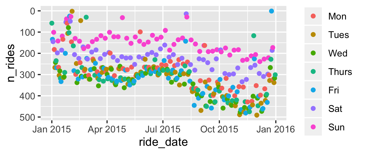<!-- --> --- ## Scale transformation ```r ggplot(data = daily, aes(x = ride_date, y = n_rides, color = day_of_week)) + geom_point() + scale_y_sqrt() ``` 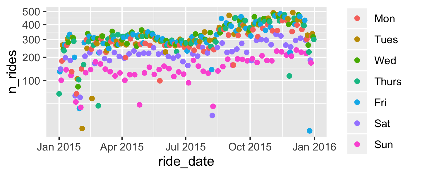<!-- --> --- ## Scale details ```r ggplot(data = daily, aes(x = ride_date, y = n_rides, color = day_of_week)) + geom_point() + scale_y_continuous(breaks = c(0, 200, 500)) ``` <!-- --> --- class: center, middle # Themes and refinements --- ## Overall themes ```r ggplot(data = daily, aes(x = ride_date, y = n_rides, color = day_of_week)) + geom_point() + theme_bw() ``` <!-- --> --- ## Overall themes ```r ggplot(data = daily, aes(x = ride_date, y = n_rides, color = day_of_week)) + geom_point() + theme_dark() ``` <!-- --> --- ## Customizing theme elements ```r ggplot(data = daily, aes(x = ride_date, y = n_rides, color = day_of_week)) + geom_point() + theme(axis.text.x = element_text(angle = 90)) ``` <!-- --> --- **Exercise 6:** Fix the axis labels in the following plot so they don't overlap by playing around with their orientation. ```r ggplot(durham_voters_summary, aes(x = age, y = n_all_voters)) + geom_bar(stat = "identity") + facet_grid(race_code ~ gender_code, scales = "free_y") ``` <!-- --> --- ## Themes Vignette To really master themes: [ggplot2.tidyverse.org/articles/extending-ggplot2.html#creating-your-own-theme](https://ggplot2.tidyverse.org/articles/extending-ggplot2.html#creating-your-own-theme) --- class: center, middle # Recap --- ## The basics * map variables to aethestics * add "geoms" for visual representation layers * scales can be independently managed * legends are automatically created * statistics are sometimes calculated by geoms --- ## Learn more * Books: - [R for Data Science](https://r4ds.had.co.nz) by Grolemund and Wickham - [R Graphics Cookbook](http://www.cookbook-r.com/Graphs/) by Chang - [Data Visualization: A Practical Introduction](https://kieranhealy.org/publications/dataviz/) by Healy * [ggplot2.tidyverse.org](https://ggplot2.tidyverse.org/) * [ggplot2 Cheat sheet](https://github.com/rstudio/cheatsheets/blob/master/data-visualization-2.1.pdf) * Contributed extensions: [ggplot2-exts.org](http://www.ggplot2-exts.org/) --- ## Thanks Thanks to Elaine McVey and Sheila Saia of R-Ladies RTP for the data!