02 teaching the tidyverse

# 02 <br> teaching the tidyverse
## 🧹 tidy up your teaching! <br> 🔗 <a href="http://bit.ly/design-ds-eku-web">bit.ly/design-ds-eku-web</a>
### dr. mine çetinkaya-rundel
### 2 april 2021

---

# What, why, how?

---

# What is the tidyverse?

---

## What is the tidyverse?

The tidyverse is an opinionated collection of R packages designed for data science. All packages share an underlying design philosophy, grammar, and data structures.

- **ggplot2** - data visualisation
- **dplyr** - data manipulation
- **tidyr** - tidy data
- **readr** - read rectangular data
- **purrr** - functional programming
- **tibble** - modern data frames
- **stringr** - string manipulation
- **forcats** - factors

---

## Tidy data

1. Each variable must have its own column.
1. Each observation must have its own row.
1. Each value must have its own cell.

---

## Pipe operator

> I want to find my keys, then start my car, then drive to work, then park my car.

- Nested

```r
park(drive(start_car(find("keys")), to = "work"))
```

- **Piped**

```r
find("keys") %>%
  start_car() %>%
  drive(to = "work") %>%
  park()
```

---

## Tidyverse references

.pull-left[
<img src="img/tidy-papers.png" width="458" />
]
.pull-right[
- Wickham, H. (2014). **Tidy data.** Journal of Statistical Software, 59(10), 1-23.
- Wickham, H., Averick, M., Bryan, J., Chang, W., McGowan, L., François, R., ... & Kuhn, M. (2019). **Welcome to the Tidyverse.** Journal of Open Source Software, 4(43), 1686.
]

---

# Why tidyverse?

---

## Recoding a binary variable

```r
mtcars$transmission <-
  ifelse(mtcars$am == 0,
         "automatic",
         "manual")
```
]
.pull-right[
### Tidyverse

```r
mtcars <- mtcars %>%
  mutate(
    transmission =
      case_when(
    am == 0 ~ "automatic",
    am == 1 ~ "manual"
    )
  )
```
]

---

## Recoding a multi-level variable

```r
mtcars$gear_char <-
  ifelse(mtcars$gear == 3,
    "three",
    ifelse(mtcars$gear == 4,
      "four",
      "five"))
```
]
.pull-right[
### Tidyverse

```r
mtcars <- mtcars %>%
  mutate(
    gear_char =
      case_when(
    gear == 3 ~ "three",
    gear == 4 ~ "four",
    gear == 5 ~ "five"
    )
  )
```
]

---

## Visualising multiple variables

### Base R

```r
mtcars$trans_color <- ifelse(mtcars$transmission == "automatic", "green", "blue")
par(mar = c(2.5, 2.5, 0, 0), mgp = c(1.5, 0.5, 0))
plot(mtcars$mpg ~ mtcars$disp, col = mtcars$trans_color)
legend("topright", legend = c("automatic", "manual"),
       pch = 1, col = c("green", "blue"))
```

![](02-teach-tidyverse_files/figure-html/unnamed-chunk-9-1.png)
]

---

## Visualising multiple variables

### Tidyverse

```r
ggplot(mtcars,
       aes(x = disp, y = mpg, color = transmission)) +
  geom_point()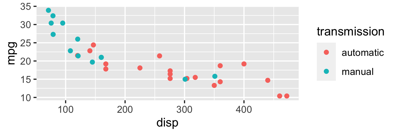
```

![](02-teach-tidyverse_files/figure-html/unnamed-chunk-10-1.png)

---

## Visualising even more variables

### Base R

```r
mtcars_cyl4 = mtcars[mtcars$cyl == 4, ]
mtcars_cyl6 = mtcars[mtcars$cyl == 6, ]
mtcars_cyl8 = mtcars[mtcars$cyl == 8, ]
par(mfrow = c(1, 3), mar = c(2.5, 2.5, 2, 0), mgp = c(1.5, 0.5, 0))
plot(mpg ~ disp, data = mtcars_cyl4, col = trans_color, main = "Cyl 4")
plot(mpg ~ disp, data = mtcars_cyl6, col = trans_color, main = "Cyl 6")
plot(mpg ~ disp, data = mtcars_cyl8, col = trans_color, main = "Cyl 8")
legend("topright", legend = c("automatic", "manual"),
       pch = 1, col = c("green", "blue"))
```

![](02-teach-tidyverse_files/figure-html/unnamed-chunk-11-1.png)
]

---

## Visualising even more variables

### Tidyverse

```r
ggplot(mtcars,
       aes(x = disp, y = mpg, color = transmission)) +
  geom_point() +
  facet_wrap(~ cyl)
```

![](02-teach-tidyverse_files/figure-html/unnamed-chunk-12-1.png)

---

## Benefits of starting with the tidyverse

- (Closer to) human readable
- Consistent syntax
- Ease of multivariate visualizations
- Data tidying/rectangling without advanced programming
- Growth opportunities:
  - dplyr -> SQL
  - purrr -> functional programming

---

# How tidyverse?

---

.discussion[
How do you start your lessons? Why?
- `library(tidyverse)` 
- `library(ggplot2)`, `library(dplyr)`, etc.
]

---

### .pink[ Sample slide ]

## ggplot2 `$\in$` tidyverse

.pull-left[
<img src="img/ggplot2-part-of-tidyverse.png" width="80%" />
]
.pull-right[
- **ggplot2** is tidyverse's data visualization package
- The `gg` in "ggplot2" stands for Grammar of Graphics
- It is inspired by the book **Grammar of Graphics** by Leland Wilkinson
]

---

# Start with ggplot2

---

## Why start with ggplot2?

1. Students come in with intuition for being able to interpret data visualizations without needing much instructions. 
  - Focus the majority of class time initially on R syntax and leave interpretations to students. 
  - Later on the scale tips -- spend more class time on concepts and results interpretations and less on R syntax.

1. It can be easier for students to detect mistakes in visualisations compared to those in data wrangling or statistical modeling. 
  
---

**Ex 1. It can be more difficult, especially for a new learner, to catch errors in data wrangling than in a data visualisation.**

Suppose we want to find the average mileage of cars with more than 100 horsepower.

- Left: Incorrect because `hp` is numeric, so no filtering is done, but also no error is given.
- Right: Correct, and note that reported mean is different.

```r
mtcars %>%
  filter(hp > "100") %>%
  summarise(mean(mpg))
```

```
##   mean(mpg)
## 1  20.09062
```
]
.pull-right[

```r
mtcars %>%
  filter(hp > 100) %>%
  summarise(mean(mpg))
```

```
##   mean(mpg)
## 1  17.45217
```
]
]

---

**Ex 2. It can be difficult to catch modeling errors, again especially for new learners.**

Fit a model predicting gas efficiency (`mpg`) from engine (`vs`, where `0` means V-shaped and `1` means straight). 
- Left: Incorrect, fit model where `vs` numeric
- Right: Correct, fit model where `vs` factor (categorical)
- Note: Slope estimates same.

```r
lm(mpg ~ vs, data = mtcars)
```

```
##         term  estimate
##  (Intercept) 16.616667
##           vs  7.940476
```
]
.pull-right[

```r
lm(mpg ~ as.factor(vs), data = mtcars)
```

```
##            term  estimate
##     (Intercept) 16.616667
##  as.factor(vs)1  7.940476
```
]
]

---

**Ex 2. Continued**

Predict `mpg` from `gear` (the number of forward gears)

- Note: slope estimates are different for numeric (left) vs. categorical (right) `gear`
- Reason for difference may be obvious to someone who is already familiar with modeling and dummy variable encoding, but not to new learners

```r
lm(mpg ~ gear, data = mtcars)
```

```
##         term estimate
##  (Intercept) 5.623333
##         gear 3.923333
```
]
.pull-right[

```r
lm(mpg ~ as.factor(gear), data = mtcars)
```

```
##              term  estimate
##       (Intercept) 16.106667
##  as.factor(gear)4  8.426667
##  as.factor(gear)5  5.273333
```
]
]

---

- If yes, do you have other reasons than the ones we listed?
- If no, why not? Are you now convinced otherwise?
]

---

# Teaching the tidyverse in 2021

---

# Reshaping data

---

## Instructional staff employment trends

The American Association of University Professors (AAUP) is a nonprofit membership association of faculty and other academic professionals. [This report](https://www.aaup.org/sites/default/files/files/AAUP_Report_InstrStaff-75-11_apr2013.pdf) by the AAUP shows trends in instructional staff employees between 1975 and 2011, and contains an image very similar to the one given below.

---

## Data

Each row in this dataset represents a faculty type, and the columns are the 
years for which we have data. The values are percentage of hires of that type 
of faculty for each year.

```r
staff <- read_csv("data/instructional-staff.csv")
staff
```

```
## # A tibble: 5 x 12
##   faculty_type                       `1975` `1989` `1993` `1995` `1999` `2001` `2003` `2005` `2007` `2009` `2011`
##   <chr>                               <dbl>  <dbl>  <dbl>  <dbl>  <dbl>  <dbl>  <dbl>  <dbl>  <dbl>  <dbl>  <dbl>
## 1 Full-Time Tenured Faculty            29     27.6   25     24.8   21.8   20.3   19.3   17.8   17.2   16.8   16.7
## 2 Full-Time Tenure-Track Faculty       16.1   11.4   10.2    9.6    8.9    9.2    8.8    8.2    8      7.6    7.4
## 3 Full-Time Non-Tenure-Track Faculty   10.3   14.1   13.6   13.6   15.2   15.5   15     14.8   14.9   15.1   15.4
## 4 Part-Time Faculty                    24     30.4   33.1   33.2   35.5   36     37     39.3   40.5   41.1   41.3
## 5 Graduate Student Employees           20.5   16.5   18.1   18.8   18.7   19     20     19.9   19.5   19.4   19.3
```
]

---

## Recreate the visualization

- In order to recreate this visualization we need to first reshape the data:
  - one variable for faculty type 
  - one variable for year
- Convert the data from the wide format to long format

- `gather()`/`spread()`
- `pivot_wider()`/ `pivot_longer()`
- Something else?
]

---

---

## `pivot_*()` functions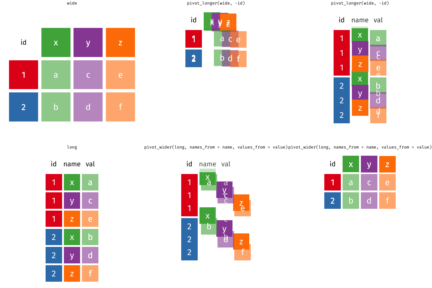

![](img/tidyr-longer-wider.gif)

---

But before we do so...

**Question:** If the long data will have a row for each year/faculty type combination, and there are 5 faculty types and 11 years of data, how many rows will the data have?

---

## `pivot_longer()`

```r
pivot_longer(
  data, 
  cols,                # columns to pivot
  names_to = "name",   # name of new column for variable names
  values_to = "value"  # name of new column for values
  )
```

---

- Go to [bit.ly/design-ds-eku](http://bit.ly/design-ds-eku) to join the RStudio Cloud workspace for this workshop
- Start the **assignment** called **02 - Teaching the tidyverse**
- Open the R Markdown document called `pivot.Rmd`, knit the document, view the result
- Convert the data from wide format to long format.
- **Stretch goal:** Convert the back to wide format from long format.
]

---

## Pivot staff data

```r
staff_long <- staff %>%
  pivot_longer(
    cols = -faculty_type, 
    names_to = "year", 
    values_to = "percentage"
    ) %>%
  mutate(percentage = as.numeric(percentage))

staff_long
```

```
## # A tibble: 55 x 3
##    faculty_type              year  percentage
##    <chr>                     <chr>      <dbl>
##  1 Full-Time Tenured Faculty 1975        29  
##  2 Full-Time Tenured Faculty 1989        27.6
##  3 Full-Time Tenured Faculty 1993        25  
##  4 Full-Time Tenured Faculty 1995        24.8
##  5 Full-Time Tenured Faculty 1999        21.8
##  6 Full-Time Tenured Faculty 2001        20.3
##  7 Full-Time Tenured Faculty 2003        19.3
##  8 Full-Time Tenured Faculty 2005        17.8
##  9 Full-Time Tenured Faculty 2007        17.2
## 10 Full-Time Tenured Faculty 2009        16.8
## # … with 45 more rows
```
]

---

## Nope!

```r
ggplot(staff_long, aes(x = percentage, y = year, color = faculty_type)) +
  geom_col(position = "dodge")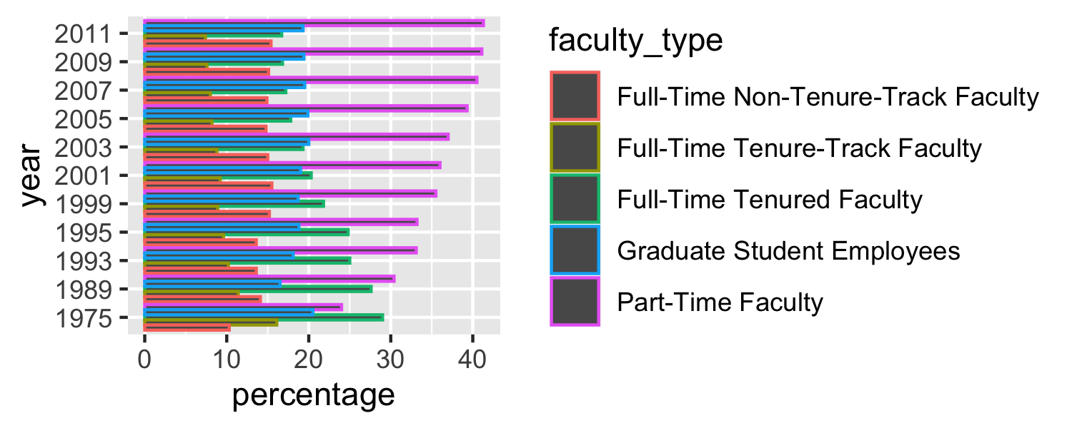
```

![](02-teach-tidyverse_files/figure-html/unnamed-chunk-22-1.png)
]

---

## Meh

```r
ggplot(staff_long, aes(x = percentage, y = year, fill = faculty_type)) +
  geom_col(position = "dodge")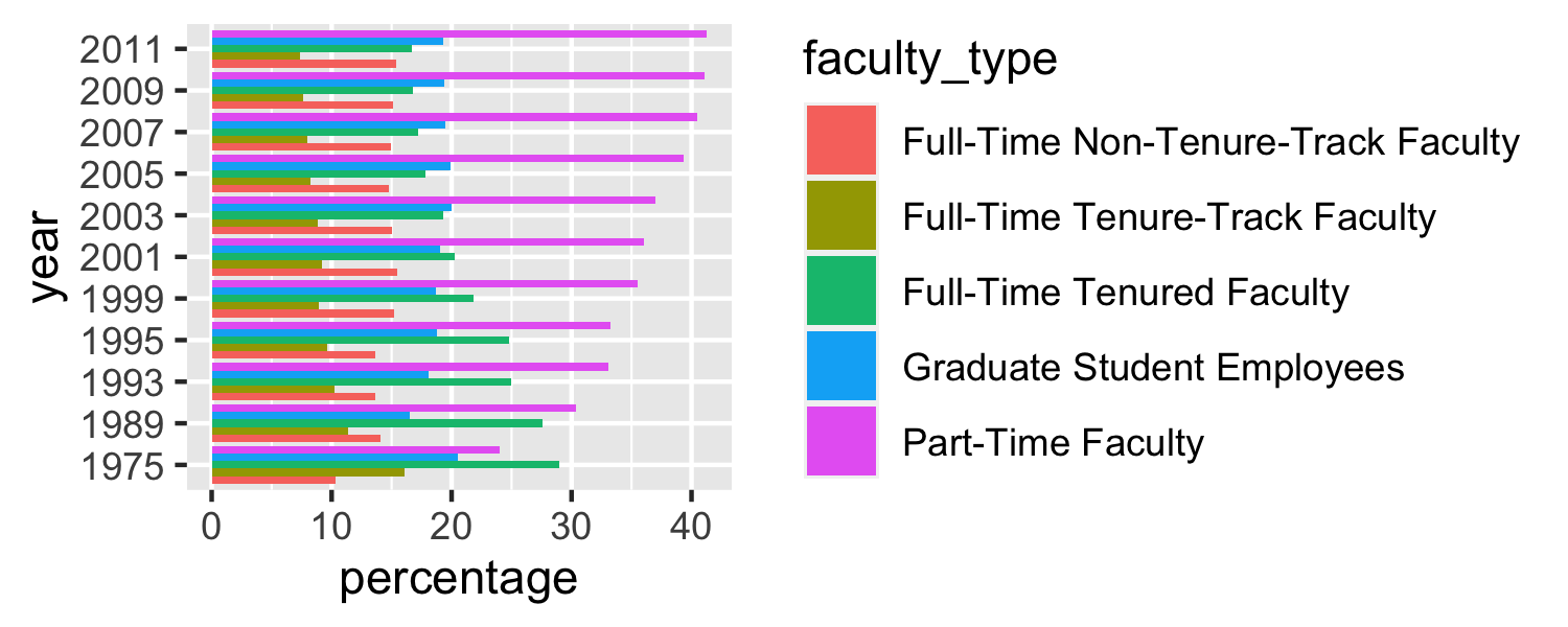
```

![](02-teach-tidyverse_files/figure-html/unnamed-chunk-23-1.png)
]

---

## Some improvement...

```r
ggplot(staff_long, aes(x = percentage, y = year, fill = faculty_type)) +
  geom_col()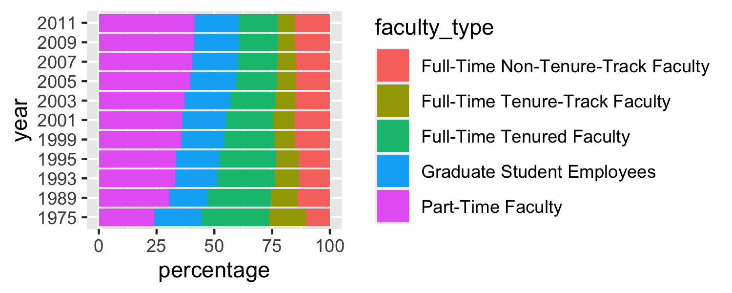
```

![](02-teach-tidyverse_files/figure-html/unnamed-chunk-24-1.png)
]

---

## More improvement

```r
ggplot(staff_long, aes(x = year, y = percentage, 
                       group = faculty_type, color = faculty_type)) +
  geom_line() +
  theme_minimal()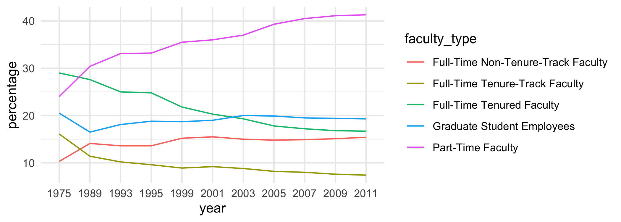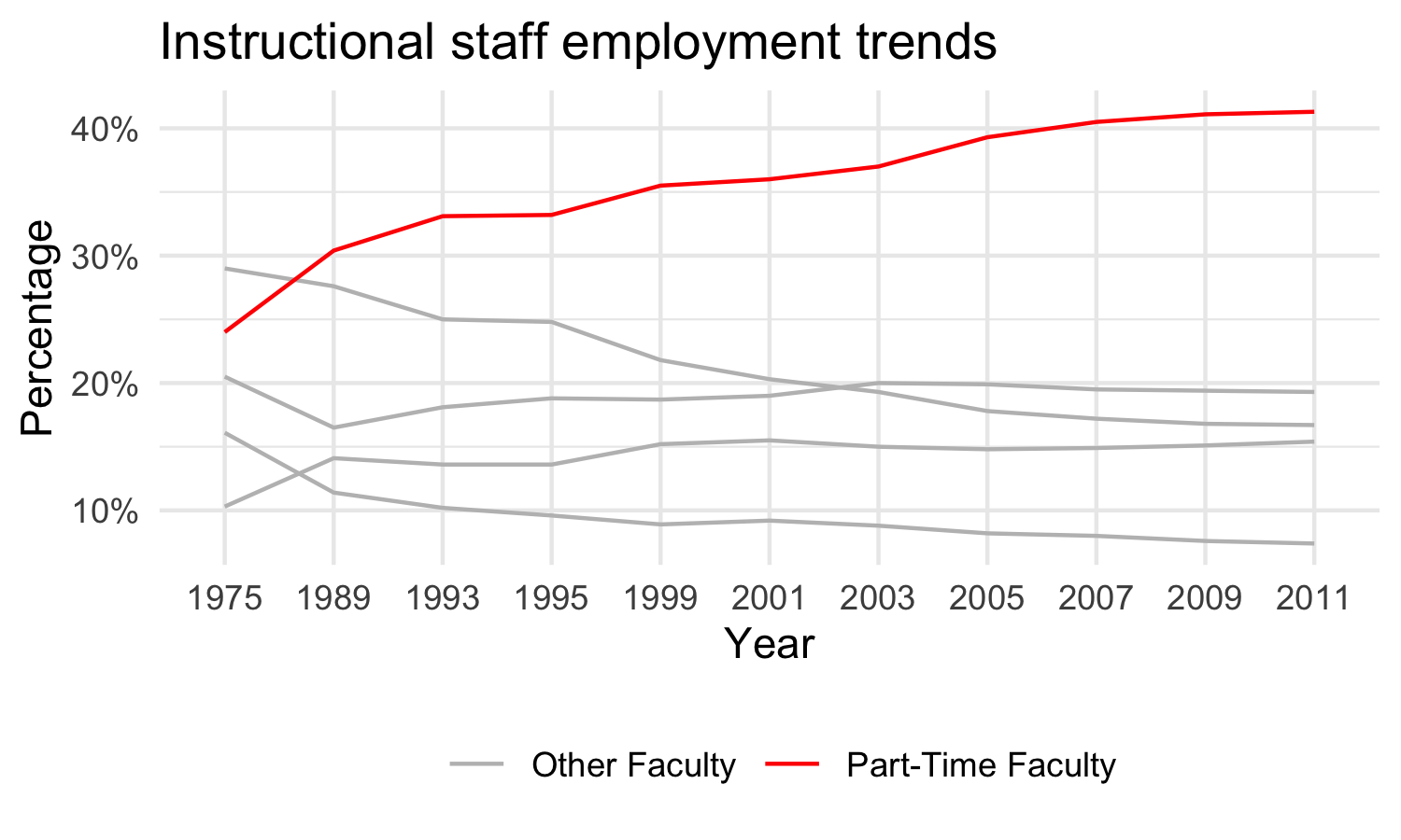
```

![](02-teach-tidyverse_files/figure-html/unnamed-chunk-25-1.png)
]

---

![](02-teach-tidyverse_files/figure-html/staff-lines-1-1.png)

---

```r
staff_long %>%
* mutate(
*   part_time = if_else(faculty_type == "Part-Time Faculty",
*                       "Part-Time Faculty", "Other Faculty"),
*   ) %>%
  ggplot(aes(x = year, y = percentage/100, group = faculty_type, 
             color = part_time)) +
  geom_line() +
* scale_color_manual(values = c("gray", "red")) +
* scale_y_continuous(labels = label_percent(accuracy = 1)) +
  theme_minimal() +
  labs(
    title = "Instructional staff employment trends",
    x = "Year", y = "Percentage", color = NULL
  ) +
  theme(legend.position = "bottom")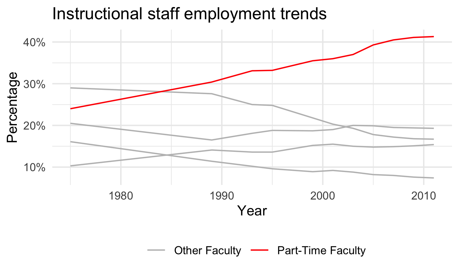
```
]

---

![](02-teach-tidyverse_files/figure-html/staff-lines-2-1.png)

---

```r
staff_long %>%
  mutate( 
    part_time = if_else(faculty_type == "Part-Time Faculty",
                        "Part-Time Faculty", "Other Faculty"),
*   year = as.numeric(year)
    ) %>% 
  ggplot(aes(x = year, y = percentage/100, group = faculty_type, 
             color = part_time)) +
  geom_line() +
  scale_color_manual(values = c("gray", "red")) + 
  scale_y_continuous(labels = label_percent(accuracy = 1)) + 
  theme_minimal() +
  labs(
    title = "Instructional staff employment trends",
    x = "Year", y = "Percentage", color = NULL
  ) +
  theme(legend.position = "bottom")
```
]

---

# Columnwise operations

---

.your-turn[
- Go to [bit.ly/design-ds-eku](http://bit.ly/design-ds-eku) to join the RStudio Cloud workspace for this workshop
- Start the **assignment** called **02 - Teaching the tidyverse**
- Open the R Markdown document called `evals.Rmd`, knit the document, view the result
- Convert all factor variables in `evals` to characters. Keep in mind that this should be introductory audience friendly, if possible. For any function you choose, think about how you would introduce it to your students.
]

---

## So long `mutate_*()`, hello `across()`

- `across()` makes it easy to apply the same transformation to multiple columns, allowing you to use `select() `semantics inside in `summarise()` and `mutate()`
- `across()` supersedes the family of *scoped variants* like `summarise_at()`, ``summarise_if()`, and `summarise_all()`

---

## Select with `where()`

```r
evals %>%
  select(where(is.factor))
```

```
## # A tibble: 463 x 9
##    rank         ethnicity    gender language cls_level cls_profs cls_credits  pic_outfit pic_color
##    <fct>        <fct>        <fct>  <fct>    <fct>     <fct>     <fct>        <fct>      <fct>    
##  1 tenure track minority     female english  upper     single    multi credit not formal color    
##  2 tenure track minority     female english  upper     single    multi credit not formal color    
##  3 tenure track minority     female english  upper     single    multi credit not formal color    
##  4 tenure track minority     female english  upper     single    multi credit not formal color    
##  5 tenured      not minority male   english  upper     multiple  multi credit not formal color    
##  6 tenured      not minority male   english  upper     multiple  multi credit not formal color    
##  7 tenured      not minority male   english  upper     multiple  multi credit not formal color    
##  8 tenured      not minority male   english  upper     single    multi credit not formal color    
##  9 tenured      not minority male   english  upper     single    multi credit not formal color    
## 10 tenured      not minority female english  upper     single    multi credit not formal color    
## # … with 453 more rows
```
]

---

## Solve with `across()`

```r
evals %>%
  mutate(across(where(is.factor), as.character))
```

```
## # A tibble: 463 x 23
##    course_id prof_id score rank       ethnicity   gender language   age cls_perc_eval cls_did_eval cls_students cls_level
##        <int>   <int> <dbl> <chr>      <chr>       <chr>  <chr>    <int>         <dbl>        <int>        <int> <chr>    
##  1         1       1   4.7 tenure tr… minority    female english     36          55.8           24           43 upper    
##  2         2       1   4.1 tenure tr… minority    female english     36          68.8           86          125 upper    
##  3         3       1   3.9 tenure tr… minority    female english     36          60.8           76          125 upper    
##  4         4       1   4.8 tenure tr… minority    female english     36          62.6           77          123 upper    
##  5         5       2   4.6 tenured    not minori… male   english     59          85             17           20 upper    
##  6         6       2   4.3 tenured    not minori… male   english     59          87.5           35           40 upper    
##  7         7       2   2.8 tenured    not minori… male   english     59          88.6           39           44 upper    
##  8         8       3   4.1 tenured    not minori… male   english     51         100             55           55 upper    
##  9         9       3   3.4 tenured    not minori… male   english     51          56.9          111          195 upper    
## 10        10       4   4.5 tenured    not minori… female english     40          87.0           40           46 upper    
## # … with 453 more rows, and 11 more variables: cls_profs <chr>, cls_credits <chr>, bty_f1lower <int>, bty_f1upper <int>,
## #   bty_f2upper <int>, bty_m1lower <int>, bty_m1upper <int>, bty_m2upper <int>, bty_avg <dbl>, pic_outfit <chr>,
## #   pic_color <chr>
```
]

---

# Rowwise operations

---

## Rowwise operations

- Lots of discussion around how to do these in the tidyverse, see [github.com/jennybc/row-oriented-workflows](https://github.com/jennybc/row-oriented-workflows) for in depth coverage

- Sometimes you need to do a simple thing, e.g. taking average of repeated measures recorded in columns in a data frame

```r
evals %>% select(score, starts_with("bty_"))
```

```
## # A tibble: 463 x 8
##    score bty_f1lower bty_f1upper bty_f2upper bty_m1lower bty_m1upper bty_m2upper bty_avg
##    <dbl>       <int>       <int>       <int>       <int>       <int>       <int>   <dbl>
##  1   4.7           5           7           6           2           4           6    5   
##  2   4.1           5           7           6           2           4           6    5   
##  3   3.9           5           7           6           2           4           6    5   
##  4   4.8           5           7           6           2           4           6    5   
##  5   4.6           4           4           2           2           3           3    3   
##  6   4.3           4           4           2           2           3           3    3   
##  7   2.8           4           4           2           2           3           3    3   
##  8   4.1           5           2           5           2           3           3    3.33
##  9   3.4           5           2           5           2           3           3    3.33
## 10   4.5           2           5           4           3           3           2    3.17
## # … with 453 more rows
```
]

---

## `rowwise()` to the rescue

Again, with the dev version of dplyr for now...

```r
evals %>%
  rowwise() %>%
  mutate(bty_avg = mean(c(bty_f1lower, bty_f1upper, bty_f2upper, bty_m1lower, bty_m1upper, bty_m2upper))) %>%
  ungroup() %>%
  select(starts_with("bty_"))
```

```
## # A tibble: 463 x 7
##    bty_f1lower bty_f1upper bty_f2upper bty_m1lower bty_m1upper bty_m2upper bty_avg
##          <int>       <int>       <int>       <int>       <int>       <int>   <dbl>
##  1           5           7           6           2           4           6    5   
##  2           5           7           6           2           4           6    5   
##  3           5           7           6           2           4           6    5   
##  4           5           7           6           2           4           6    5   
##  5           4           4           2           2           3           3    3   
##  6           4           4           2           2           3           3    3   
##  7           4           4           2           2           3           3    3   
##  8           5           2           5           2           3           3    3.33
##  9           5           2           5           2           3           3    3.33
## 10           2           5           4           3           3           2    3.17
## # … with 453 more rows
```
]

---

# When to purrr?

---

.discussion[
How familiar are you with the purrr package? Do you teach it in your introductory data science courses? If yes, how much?
]

---

## Ex 1. Flattening JSON files

We have data on lego sales and some information on the buyers in JSON format. We want to covert it into a tidy data frame.

```
## [
##   {
##     "gender": ["Female"],
##     "first_name": ["Kimberly"],
##     "last_name": ["Beckstead"],
##     "age": [24],
##     "phone_number": ["216-555-2549"],
##     "hobbies": ["Ultimate Disc", "Shopping"],
##     "purchases": [
##       {
##         "SetID": [24701],
##         "Number": ["76062"],
##         "Theme": ["DC Comics Super Heroes"],
##         "Subtheme": ["Mighty Micros"],
##         "Year": [2016],
##         "Name": ["Robin vs. Bane"],
##         "Pieces": [77],
##         "USPrice": [9.99],
##         "ImageURL": ["http://images.brickset.com/sets/images/76062-1.jpg"],
##         "Quantity": [1]
##       }
##     ]
##   }
## ]
```
]

---

## purrr solution

```r
sales %>%
  purrr::map_dfr(
    function(l) {
      purchases <- purrr::map_dfr(l$purchases, ~.)
      
      l$purchases <- NULL
      l$hobbies <- list(l$hobbies)
      
      cbind(as_tibble(l), purchases) %>% as_tibble()
    }
  )
```

---

## purr solution

```
## # A tibble: 620 x 16
##    gender first_name last_name   age phone_number hobbies SetID Number Theme Subtheme  Year Name  Pieces USPrice ImageURL
##    <chr>  <chr>      <chr>     <dbl> <chr>        <list>  <int> <chr>  <chr> <chr>    <int> <chr>  <int>   <dbl> <chr>   
##  1 Female Kimberly   Beckstead    24 216-555-2549 <chr [… 24701 76062  DC C… "Mighty…  2016 Robi…     77    9.99 http://…
##  2 Male   Neel       Garvin       35 819-555-3189 <chr [… 25626 70595  Ninj… "Rise o…  2016 Ultr…   1093  120.   http://…
##  3 Male   Neel       Garvin       35 819-555-3189 <chr [… 24665 21031  Arch… ""        2016 Burj…    333   40.0  http://…
##  4 Female Chelsea    Bouchard     41 <NA>         <chr [… 24695 31048  Crea… ""        2016 Lake…    368   30.0  http://…
##  5 Female Chelsea    Bouchard     41 <NA>         <chr [… 25626 70595  Ninj… "Rise o…  2016 Ultr…   1093  120.   http://…
##  6 Female Chelsea    Bouchard     41 <NA>         <chr [… 24721 10831  Duplo ""        2016 My F…     19    9.99 http://…
##  7 Female Bryanna    Welsh        19 <NA>         <chr [… 24797 75138  Star… "Episod…  2016 Hoth…    233   25.0  http://…
##  8 Female Bryanna    Welsh        19 <NA>         <chr [… 24701 76062  DC C… "Mighty…  2016 Robi…     77    9.99 http://…
##  9 Male   Caleb      Garcia-W…    37 907-555-9236 <chr [… 24730 41115  Frie… ""        2016 Emma…    108    9.99 http://…
## 10 Male   Caleb      Garcia-W…    37 907-555-9236 <chr [… 25611 21127  Mine… "Minifi…  2016 The …     NA  110.   http://…
## # … with 610 more rows, and 1 more variable: Quantity <dbl>
```

---

## tidyr solution

```r
sales %>%
  tibble(sales = .) %>%
  unnest_wider(sales) %>%
  unnest_longer(purchases) %>%
  unnest_wider(purchases)
```

---

## tidyr solution - Step 1

```r
sales %>%
  tibble(sales = .)
```

```
## # A tibble: 250 x 1
##    sales           
##    <list>          
##  1 <named list [7]>
##  2 <named list [7]>
##  3 <named list [6]>
##  4 <named list [6]>
##  5 <named list [7]>
##  6 <named list [7]>
##  7 <named list [7]>
##  8 <named list [7]>
##  9 <named list [7]>
## 10 <named list [7]>
## # … with 240 more rows
```
]

---

## tidyr solution - Step 2

```r
sales %>%
  tibble(sales = .) %>%
  unnest_wider(sales)
```

```
## # A tibble: 250 x 7
##    gender first_name last_name        age phone_number hobbies   purchases 
##    <chr>  <chr>      <chr>          <dbl> <chr>        <list>    <list>    
##  1 Female Kimberly   Beckstead         24 216-555-2549 <chr [2]> <list [1]>
##  2 Male   Neel       Garvin            35 819-555-3189 <chr [2]> <list [2]>
##  3 Female Chelsea    Bouchard          41 <NA>         <chr [3]> <list [3]>
##  4 Female Bryanna    Welsh             19 <NA>         <chr [2]> <list [2]>
##  5 Male   Caleb      Garcia-Wideman    37 907-555-9236 <chr [3]> <list [2]>
##  6 Male   Chase      Fortenberry       19 205-555-3704 <chr [2]> <list [2]>
##  7 Male   Kevin      Cruz              20 947-555-7946 <chr [1]> <list [1]>
##  8 Male   Connor     Brown             36 516-555-4310 <chr [1]> <list [3]>
##  9 Female Toni       Borison           40 284-555-4560 <chr [2]> <list [2]>
## 10 Male   Daniel     Hurst             44 251-555-0845 <chr [1]> <list [2]>
## # … with 240 more rows
```
]

---

## tidyr solution - Step 3

```r
sales %>%
  tibble(sales = .) %>%
  unnest_wider(sales) %>%
  unnest_longer(purchases)
```

```
## # A tibble: 620 x 7
##    gender first_name last_name        age phone_number hobbies   purchases        
##    <chr>  <chr>      <chr>          <dbl> <chr>        <list>    <list>           
##  1 Female Kimberly   Beckstead         24 216-555-2549 <chr [2]> <named list [10]>
##  2 Male   Neel       Garvin            35 819-555-3189 <chr [2]> <named list [10]>
##  3 Male   Neel       Garvin            35 819-555-3189 <chr [2]> <named list [10]>
##  4 Female Chelsea    Bouchard          41 <NA>         <chr [3]> <named list [10]>
##  5 Female Chelsea    Bouchard          41 <NA>         <chr [3]> <named list [10]>
##  6 Female Chelsea    Bouchard          41 <NA>         <chr [3]> <named list [10]>
##  7 Female Bryanna    Welsh             19 <NA>         <chr [2]> <named list [10]>
##  8 Female Bryanna    Welsh             19 <NA>         <chr [2]> <named list [10]>
##  9 Male   Caleb      Garcia-Wideman    37 907-555-9236 <chr [3]> <named list [10]>
## 10 Male   Caleb      Garcia-Wideman    37 907-555-9236 <chr [3]> <named list [10]>
## # … with 610 more rows
```
]

---

## tidyr solution - Step 4

```r
sales %>%
  tibble(sales = .) %>%
  unnest_wider(sales) %>%
  unnest_longer(purchases) %>%
  unnest_wider(purchases)
```

---

## tidyr solution - Auto

```r
sales %>%
  tibble(sales = .) %>%
  unnest_auto(sales) %>%
  unnest_auto(purchases) %>%
  unnest_auto(purchases)
```

```
## Using `unnest_wider(sales)`; elements have 6 names in common
```

```
## Using `unnest_longer(purchases)`; no element has names
```

```
## Using `unnest_wider(purchases)`; elements have 10 names in common
```

---

## Moral of the story

- There are many ways of getting to the answer
- Some likely need more scaffolding than others
- It's worth considering how much of `purrr` fits into your introductory data science curriculum
  - We'll give one example later where `purrr` provides big wins in the context of web scraping from many, similarly formatted pages!

---

# A vast tidy ecosystem

---

## tidyverse friendly packages

- [**janitor**](https://garthtarr.github.io/meatR/janitor.html)
- [**kableExtra**](https://cran.r-project.org/web/packages/kableExtra/vignettes/awesome_table_in_html.html)
- [**patchwork**](https://patchwork.data-imaginist.com/)
- [**gghighlight**](https://cran.r-project.org/web/packages/gghighlight/vignettes/gghighlight.html)

---

## janitor

```
## # A tibble: 3 x 3
##      ID patientName blood.pressure
##   <int> <chr>       <chr>         
## 1     1 A           120/80        
## 2     2 B           130/90        
## 3     3 C           120/85
```
]

```r
library(janitor)
df %>%
  clean_names()
```

```
## # A tibble: 3 x 3
##      id patient_name blood_pressure
##   <int> <chr>        <chr>         
## 1     1 A            120/80        
## 2     2 B            130/90        
## 3     3 C            120/85
```
]

---

## kableExtra

```r
library(kableExtra)
df %>%
  clean_names() %>%
  kbl(caption = "Recreating booktabs style table") %>%
  kable_classic_2(full_width = F, html_font = "Cambria")
```

<table class=" lightable-classic-2" style="font-family: Cambria; width: auto !important; margin-left: auto; margin-right: auto;">
<caption>Recreating booktabs style table</caption>
 <thead>
  <tr>
   <th style="text-align:right;"> id </th>
   <th style="text-align:left;"> patient_name </th>
   <th style="text-align:left;"> blood_pressure </th>
  </tr>
 </thead>
<tbody>
  <tr>
   <td style="text-align:right;"> 1 </td>
   <td style="text-align:left;"> A </td>
   <td style="text-align:left;"> 120/80 </td>
  </tr>
  <tr>
   <td style="text-align:right;"> 2 </td>
   <td style="text-align:left;"> B </td>
   <td style="text-align:left;"> 130/90 </td>
  </tr>
  <tr>
   <td style="text-align:right;"> 3 </td>
   <td style="text-align:left;"> C </td>
   <td style="text-align:left;"> 120/85 </td>
  </tr>
</tbody>
</table>

---

## patchwork

```r
library(patchwork)

p1 + p2 + p3 + p4 + 
  plot_layout(widths = c(2, 1))
```

<img src="02-teach-tidyverse_files/figure-html/unnamed-chunk-45-1.png" width="100%" />
]

---

## gghighlight

```r
library(gghighlight)
library(palmerpenguins)
ggplot(penguins, aes(x = bill_length_mm, y = bill_depth_mm, color = species)) +
  geom_point() +
  theme_minimal() +
  gghighlight(bill_length_mm > 50)
```

![](02-teach-tidyverse_files/figure-html/unnamed-chunk-46-1.png)
]

---

# Resources

---

## Recommended reading

- Keep up to date with the [tidyverse blog](https://www.tidyverse.org/blog/) **for packages you teach**
- Four part blog series: Teaching the Tidyverse in 2020
  - [Part 1](https://education.rstudio.com/blog/2020/07/teaching-the-tidyverse-in-2020-part-1-getting-started/)
  - [Part 2](https://education.rstudio.com/blog/2020/07/teaching-the-tidyverse-in-2020-part-2-data-visualisation/)
  - [Part 3](https://education.rstudio.com/blog/2020/07/teaching-the-tidyverse-in-2020-part-3-data-wrangling-and-tidying/)
  - [Part 4](https://education.rstudio.com/blog/2020/07/teaching-the-tidyverse-in-2020-part-4-when-to-purrr/)